Page 122 - Schaum's Outline of Theory and Problems of Electric Circuits

WAVEFORMS AND SIGNALS
CHAP. 6]

Fig. 6-10 111

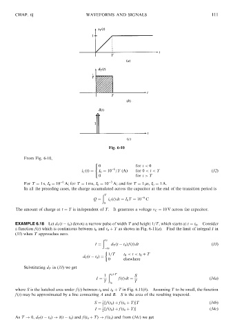
From Fig. 6-10,
8
< 0 for t < 0
6
i C ðtÞ¼ I 0 ¼ 10 =T ðAÞ for 0 < t < T ð32Þ
:
0 for t > T
For T ¼ 1s, I 0 ¼ 10 6 A; for T ¼ 1 ms, I 0 ¼ 10 3 A; and for T ¼ 1 ms, I 0 ¼ 1A.
In all the preceding cases, the charge accumulated across the capacitor at the end of the transition period is
ð T
Q ¼ i C ðtÞ dt ¼ I 0 T ¼ 10 6 C
0
The amount of charge at t ¼ T is independent of T. It generates a voltage v C ¼ 10 V across the capacitor.

EXAMPLE 6.18 Let d T ðt t 0 Þ denote a narrow pulse of width T and height 1=T, which starts at t ¼ t 0 . Consider
a function f ðtÞ which is continuous between t 0 and t 0 þ T as shown in Fig. 6-11(a). Find the limit of integral I in
(33) when T approaches zero.
ð 1
I ¼ d T ðt t 0 Þ f ðtÞ dt ð33Þ
1

1=T t 0 < t < t 0 þ T
d T ðt t 0 Þ¼
0 elsewhere
Substituting d T in (33) we get
ð
1 t 0 þT S
I ¼ f ðtÞ dt ¼ ð34aÞ
T T
t 0
where S is the hatched area under f ðtÞ between t 0 and t 0 þ T in Fig. 6.11(b). Assuming T to be small, the function
f ðtÞ may be approximated by a line connecting A and B. S is the area of the resulting trapezoid.
1
S ¼ ½ f ðt 0 Þþ f ðt 0 þ TފT ð34bÞ
2
1
I ¼ ½ f ðt 0 Þþ f ðt 0 þ Tފ ð34cÞ
2
As T ! 0, d T ðt t 0 Þ! ðt t 0 Þ and f ðt 0 þ TÞ! f ðt 0 Þ and from (34c) we get