Page 124 - Schaum's Outline of Theory and Problems of Electric Circuits

WAVEFORMS AND SIGNALS
CHAP. 6]

Fig. 6-12 113
2
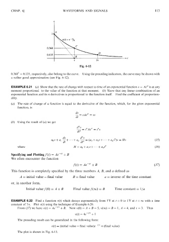
0.368 ¼ 0:135, respectively, also belong to the curve. Using the preceding indicators, the curve may be drawn with
a rather good approximation (see Fig. 6-12).

st
EXAMPLE 6.21 (a) Show that the rate of change with respect to time of an exponential function v ¼ Ae is at any
moment proportional to the value of the function at that moment. (b) Show that any linear combination of an
exponential function and its n derivatives is proportional to the function itself. Find the coefficient of proportion-
ality.
(a) The rate of change of a function is equal to the derivative of the function, which, for the given exponential
function, is
dv st
¼ sAe ¼ sv
dt
(b) Using the result of (a) we get
n
d v n st n
¼ s Ae ¼ s v
dt n
n
dv d v n
a 0 v þ a 1 þ þ a n n ¼ða 0 þ a 1 s þ þ a n s Þv ¼ Hv ð35Þ
dt dt
where H ¼ a 0 þ a 1 s þ þ a n s n (36)
Specifying and Plotting f ðtÞ¼ Ae at þ B
We often encounter the function
at
f ðtÞ¼ Ae þ B ð37Þ
This function is completely specified by the three numbers A, B,and a defined as

A ¼ initial value final value B ¼ final value a ¼ inverse of the time constant
or, in another form,
Initial value f ð0Þ¼ A þ B Final value f ð1Þ ¼ B Time constant ¼ 1=a

EXAMPLE 6.22 Find a function vðtÞ which decays exponentially from 5 V at t ¼ 0to 1 Vat t ¼1 with a time
constant of 3 s. Plot vðtÞ using the technique of Example 6.20.
t=
From (37) we have vðtÞ¼ Ae þ B. Now vð0Þ¼ A þ B ¼ 5, vð1Þ ¼ B ¼ 1, A ¼ 4, and ¼ 3. Thus
t=3
vðtÞ¼ 4e þ 1
The preceding result can be generalized in the following form:
vðtÞ¼ðinitial value final valueÞe t= þðfinal valueÞ
The plot is shown in Fig. 6-13.