Page 123 - Schaum's Outline of Theory and Problems of Electric Circuits

WAVEFORMS AND SIGNALS
112

Fig. 6-11 [CHAP. 6

1
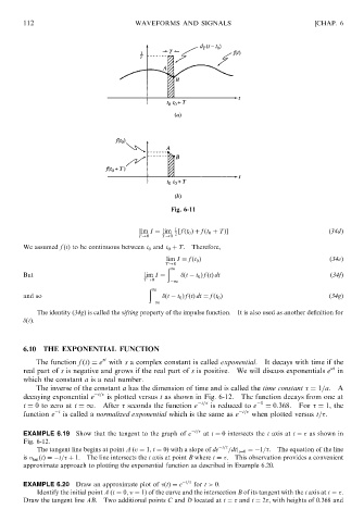
lim I ¼ lim ½ f ðt 0 Þþ f ðt 0 þ Tފ ð34dÞ
T!0 T!0 2
We assumed f ðtÞ to be continuous between t 0 and t 0 þ T. Therefore,
lim I ¼ f ðt 0 Þ ð34eÞ
T!0
ð
1
But lim I ¼ ðt t 0 Þ f ðtÞ dt (34f)
T!0 1
ð
1
and so ðt t 0 Þ f ðtÞ dt ¼ f ðt 0 Þ (34g)
1
The identity (34g) is called the sifting property of the impulse function. It is also used as another definition for
ðtÞ.

6.10 THE EXPONENTIAL FUNCTION
st
The function f ðtÞ¼ e with s a complex constant is called exponential. It decays with time if the
at
real part of s is negative and grows if the real part of s is positive. We will discuss exponentials e in
which the constant a is a real number.
The inverse of the constant a has the dimension of time and is called the time constant ¼ 1=a.A
t=
decaying exponential e is plotted versus t as shown in Fig. 6-12. The function decays from one at
t= 1
t ¼ 0 to zero at t ¼1. After seconds the function e is reduced to e ¼ 0:368. For ¼ 1, the
t t=
function e is called a normalized exponential which is the same as e when plotted versus t= .
t=
EXAMPLE 6.19 Show that the tangent to the graph of e at t ¼ 0 intersects the t axis at t ¼ as shown in
Fig. 6-12.
The tangent line begins at point A ðv ¼ 1; t ¼ 0Þ with a slope of de t= =dtj t¼0 ¼ 1= . The equation of the line
is v tan ðtÞ¼ t= þ 1. The line intersects the t axis at point B where t ¼ . This observation provides a convenient
approximate approach to plotting the exponential function as described in Example 6.20.

t=
EXAMPLE 6.20 Draw an approximate plot of vðtÞ¼ e for t > 0.
Identify the initial point A (t ¼ 0; v ¼ 1Þ of the curve and the intersection B of its tangent with the t axis at t ¼ .
Draw the tangent line AB. Two additional points C and D located at t ¼ and t ¼ 2 , with heights of 0.368 and