Page 150 - Shigley's Mechanical Engineering Design

bud29281_ch03_071-146.qxd 11/25/09 4:55PM Page 125 ntt 203:MHDQ196:bud29281:0073529281:bud29281_pagefiles:

Load and Stress Analysis 125
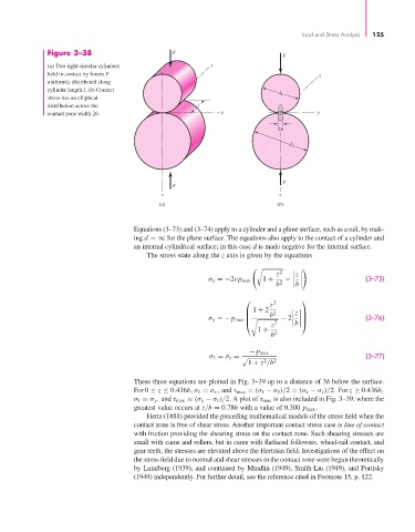
Figure 3–38 F
F
(a) Two right circular cylinders x
held in contact by forces F x
uniformly distributed along
cylinder length l. (b) Contact
d 1
stress has an elliptical
distribution across the l
contact zone width 2b. y y

2b

d 2

F
F
z z
(a) (b)

Equations (3–73) and (3–74) apply to a cylinder and a plane surface, such as a rail, by mak-
ing d =∞ for the plane surface. The equations also apply to the contact of a cylinder and
an internal cylindrical surface; in this case d is made negative for the internal surface.
The stress state along the z axis is given by the equations

z 2 z
σ x =−2νp max 1 + 2 − (3–75)
b
b
z
⎛ 2 ⎞
1 + 2
b
⎜ 2 z ⎟
σ y =−p max ⎜ − 2 ⎟ (3–76)
b
z
⎝ 2 ⎠
1 +
b 2
−p max
(3–77)
σ 3 = σ z =
1 + z /b 2
2
These three equations are plotted in Fig. 3–39 up to a distance of 3b below the surface.
For 0 ≤ z ≤ 0.436b,σ 1 = σ x , and τ max = (σ 1 − σ 3 )/2 = (σ x − σ z )/2. For z ≥ 0.436b,
σ 1 = σ y , and τ max = (σ y − σ z )/2. A plot of τ max is also included in Fig. 3–39, where the
greatest value occurs at z/b = 0.786 with a value of 0.300 p max .
Hertz (1881) provided the preceding mathematical models of the stress field when the
contact zone is free of shear stress. Another important contact stress case is line of contact
with friction providing the shearing stress on the contact zone. Such shearing stresses are
small with cams and rollers, but in cams with flatfaced followers, wheel-rail contact, and
gear teeth, the stresses are elevated above the Hertzian field. Investigations of the effect on
the stress field due to normal and shear stresses in the contact zone were begun theoretically
by Lundberg (1939), and continued by Mindlin (1949), Smith-Liu (1949), and Poritsky
(1949) independently. For further detail, see the reference cited in Footnote 15, p. 122.