Page 333 - Shigley's Mechanical Engineering Design

bud29281_ch06_265-357.qxd 12/02/2009 9:29 pm Page 308 pinnacle s-171:Desktop Folder:Temp Work:Don't Delete (Jobs):MHDQ196/Budynas:

308 Mechanical Engineering Design
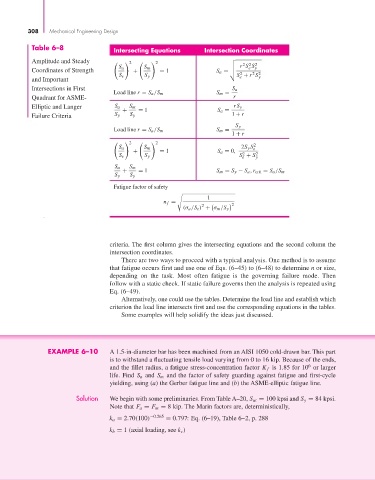
Table 6–8 Intersecting Equations Intersection Coordinates

Amplitude and Steady 2 2 2 2 2
r S S

Coordinates of Strength S a + S m = 1 S a = e y
2
2 2
S e S y S + r S y
e
and Important
Intersections in First S a
Load line r = S a /S m S m =
Quadrant for ASME- r
Elliptic and Langer S a S m rS y
+ = 1 S a =
Failure Criteria S y S y 1 + r
S y
Load line r = S a /S m S m =
1 + r
2 2
2
S a S m 2S y S e
+ = 1 S a = 0, 2 2
S e S y S + S
e y
S a S m
+ = 1 S m = S y − S a ,r crit = S a /S m
S y S y
Fatigue factor of safety

1
n f =
2 2
(σ a /S e ) + σ m /S y

criteria. The first column gives the intersecting equations and the second column the
intersection coordinates.
There are two ways to proceed with a typical analysis. One method is to assume
that fatigue occurs first and use one of Eqs. (6–45) to (6–48) to determine n or size,
depending on the task. Most often fatigue is the governing failure mode. Then
follow with a static check. If static failure governs then the analysis is repeated using
Eq. (6–49).
Alternatively, one could use the tables. Determine the load line and establish which
criterion the load line intersects first and use the corresponding equations in the tables.
Some examples will help solidify the ideas just discussed.

EXAMPLE 6–10 A 1.5-in-diameter bar has been machined from an AISI 1050 cold-drawn bar. This part
is to withstand a fluctuating tensile load varying from 0 to 16 kip. Because of the ends,
6
and the fillet radius, a fatigue stress-concentration factor K f is 1.85 for 10 or larger
life. Find S a and S m and the factor of safety guarding against fatigue and first-cycle
yielding, using (a) the Gerber fatigue line and (b) the ASME-elliptic fatigue line.

Solution We begin with some preliminaries. From Table A–20, S ut = 100 kpsi and S y = 84 kpsi.
Note that F a = F m = 8 kip. The Marin factors are, deterministically,
k a = 2.70(100) −0.265 = 0.797: Eq. (6–19), Table 6–2, p. 288
k b = 1 (axial loading, see k c )