Page 471 - Shigley's Mechanical Engineering Design

bud29281_ch08_409-474.qxd 12/16/2009 7:11 pm Page 446 pinnacle 203:MHDQ196:bud29281:0073529281:bud29281_pagefiles:

446 Mechanical Engineering Design
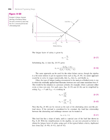
Figure 8–20
S
Designer’s fatigue diagram e
showing a Goodman failure
line and a commonly used load Load line
Alternating stress a
line for a constant preload and
a fluctuating load.

S
a
B C
a
A D
F S S
= A i t m m ut
i
Steady stress
m

The fatigue factor of safety is given by

S a
n f = (8–37)
σ a
Substituting Eq. (c) into Eq. (8–37) gives

S e (S ut − σ i )
n f = (8–38)
S ut σ a + S e (σ m − σ i )

The same approach can be used for the other failure curves, though the algebra
is a bit more tedious to put in equation form such as Eq. (8–38). An easier approach
would be to solve in stages numerically, first S m , then S a , and finally n f .
Often, the type of fatigue loading encountered in the analysis of bolted joints is one
in which the externally applied load fluctuates between zero and some maximum force P.
This would be the situation in a pressure cylinder, for example, where a pressure either
exists or does not exist. For such cases, Eqs. (8–35) and (8–36) can be simplified by
setting P max = P and P min = 0, resulting in

CP
σ a = (8–39)
2A t
CP F i
σ m = + (8–40)
2A t A t
Note that Eq. (8–40) can be viewed as the sum of the alternating stress and the pre-
load stress. If the preload is considered to be constant, the load line relationship
between the alternating and midrange stresses can be treated as

(8–41)
σ m = σ a + σ i
This load line has a slope of unity, and is a special case of the load line shown in
Fig. 8–20. With the simplifications in the algebra, we can now proceed as before to
obtain the fatigue factor of safety using each of the typical failure criteria, duplicated
here from Eqs. (6–40), (6–41), and (6–42).