Page 234 - Six Sigma Demystified

214 Six SigMa DemystifieD

Two-Sided Example at 95% Confidence

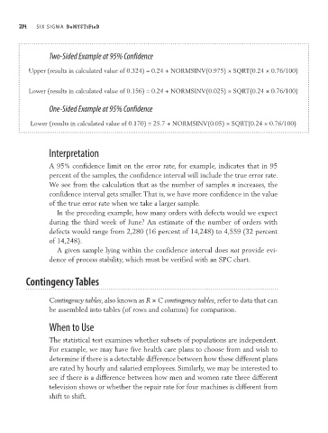
Upper (results in calculated value of 0.324) = 0.24 + NORMSINV(0.975) × SQRT(0.24 × 0.76/100)

Lower (results in calculated value of 0.156) = 0.24 + NORMSINV(0.025) × SQRT(0.24 × 0.76/100)

One-Sided Example at 95% Confidence

Lower (results in calculated value of 0.170) = 25.7 + NORMSINV(0.05) × SQRT(0.24 × 0.76/100)

Interpretation
A 95% confidence limit on the error rate, for example, indicates that in 95
percent of the samples, the confidence interval will include the true error rate.
We see from the calculation that as the number of samples n increases, the
confidence interval gets smaller. That is, we have more confidence in the value
of the true error rate when we take a larger sample.
In the preceding example, how many orders with defects would we expect
during the third week of June? An estimate of the number of orders with
defects would range from 2,280 (16 percent of 14,248) to 4,559 (32 percent
of 14,248).
A given sample lying within the confidence interval does not provide evi-
dence of process stability, which must be verified with an SPC chart.

Contingency Tables

Contingency tables, also known as R × C contingency tables, refer to data that can
be assembled into tables (of rows and columns) for comparison.

When to Use

The statistical test examines whether subsets of populations are independent.
For example, we may have five health care plans to choose from and wish to
determine if there is a detectable difference between how these different plans
are rated by hourly and salaried employees. Similarly, we may be interested to
see if there is a difference between how men and women rate three different
television shows or whether the repair rate for four machines is different from
shift to shift.