Page 235 - Six Sigma Demystified

Part 3 s i x s i g m a to o l s 215

Analyze Stage
• To compare results of sampling from different process conditions to de-
tect if they are independent

Methodology

The methodology for analyzing the R rows by C columns involves using the
chi-square statistic to compare the observed frequencies with the expected
frequencies, assuming independence of the subsets. The null hypothesis is that
the p values are equal for each column in each row. The alternative hypothesis
is that at least one of the p values is different.
Construct the R × C table by separating the subsets of the population into
the tested categories.
Calculate the expected values for each row-column intersection cell e . The
ij
expected value for each row/column is found by multiplying the percent of
that row by the percent of the column by the total number.
Calculate the test statistic:

r c (o − e ) 2
0 ∑
χ = ∑ ij ij
2
1 =
i = j 1 e ij
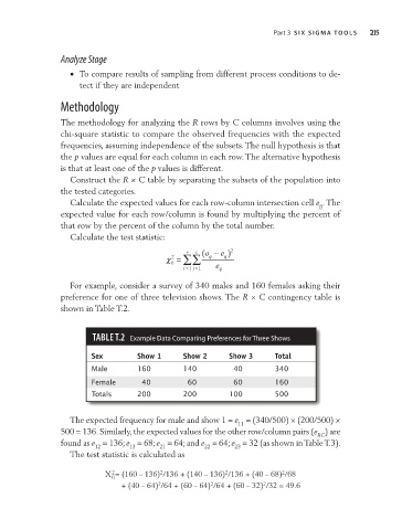
For example, consider a survey of 340 males and 160 females asking their
preference for one of three television shows. The R × C contingency table is
shown in Table T.2.

TAble T.2 Example Data Comparing Preferences for Three Shows

Sex Show 1 Show 2 Show 3 Total
Male 160 140 40 340
Female 40 60 60 160
Totals 200 200 100 500

The expected frequency for male and show 1 = e = (340/500) × (200/500) ×
11
500 = 136. Similarly, the expected values for the other row/column pairs (e ) are
RC
found as e = 136; e = 68; e = 64; and e = 64; e = 32 (as shown in Table T.3).
12
22
13
21
23
The test statistic is calculated as
2
2
X = (160 – 136) /136 + (140 – 136) /136 + (40 – 68) /68
2
2
0
2
+ (40 – 64) /64 + (60 – 64) /64 + (60 – 32) /32 = 49.6
2
2