Page 165 - Standard Handbook Of Petroleum & Natural Gas Engineering

150 General Engineering and Science

Table 2-5
One-dimensional Differential Equations of Motion and Their Solutions
Diffacluial
buations a/a = coa~tant a = a([); a = a(t) a= ~v): a= NO) a= a(s); a= 40)
'=[a
Linear

Rotafional o=dB y=q+at Or = 0, + 1; w (t) dt

to these equations are in Columns 2-5, for the cases of constant acceleration,
acceleration as a function of time, acceleration as a function of velocity, and
acceleration as a function of displacement s.
For rotational motion, as illustrated in Figure 2-6b, a completely analogous set of
equations and solutions are given in the bottom half of Table 2-5. There w is called
the angular velocity and has units of radians/s, and a is called angular acceleration
and has units of radians/s2.
The equations of Table 2-5 are all scalar equations representing discrete components
of motions along orthogonal axes. The axis along which the component w or a acts
is defined in the same fashion as for a couple. That is, the direction of w is outwardly
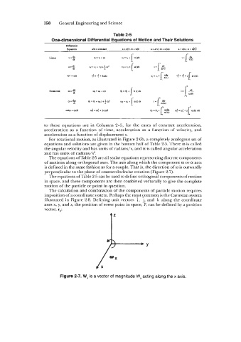
perpendicular to the plane of counterclockwise rotation (Figure 2-7).
The equations of'rable 2-5 can be used to define orthogonal components of motion
in space, and these components are then combined vectorally to give the complete
motion of the particle or point in question.
The calculation and combination of the components of particle motion requires
imposition of a coordinate system. Perhaps the most SomrnoQ is the Cartesian system
illustrated in Figure 2-8. Defining unit vectors i, j, and k along the coordinate
axes x, y, and z, the position of some point in space, P, can be defined by a position
vector, rp:

Figure 2-7. Wx is a vector of magnitude Wx acting along the x axis.