Page 137 - Statistics and Data Analysis in Geology

Statistics and Data Analysis in Geology - Chapter 5

a x2 test exactly like that used to check the fit of the Poisson model. Again, it is
necessary to combine the final three categories so a frequency of five or more is
obtained. The test statistic is x2 = 4.82, with (5 - 2 = 3) degrees of freedom. This
is less than the critical value of x2 for o( = 0.05 and v = 3, so we cannot reject
the negative binomial as a model of the spatial distribution of discovery wells in
the eastern part of the Permian Basin. Keep in mind that this is not equivalent to
proof that the wells do follow a negative binomial model, because it is possible that
some other clustered model might provide an even better fit. However, the negative
binomial does generate a spatial distribution that is statistically indistinguishable
from the one observed.

Nearest- neig h bor an a lysis
An alternative to quadrat analysis is nearest-neighbor analysis. The data used are
not the numbers of points within subareas, but the distances between closest pairs
of points. Since it is not necessary to select a quadrat size, nearest-neighbor pro-
cedures avoid the possibility of finding that a pattern is random at one scale but
not at another. Also, since there are usually many more pairs of nearest neigh-
bors than quadrats, the analysis is more sensitive. A good introduction to nearest-
neighbor techniques is given by Getis and Boots (1978). Ripley (1981) provides a
review of theory and applications in several fields, as do Cliff and Ord (1981). Shaw
and Wheeler (1994) and B&ley and Gatrell(1995) discuss computational aspects of
neares t-neighbor analyses.
Nearest-neighbor analysis compares characteristics of the observed set of dis-
tances between pairs of nearest points with those that would be expected if the
points were randomly placed. The characteristics of a theoretical random pattern
can be derived from the Poisson distribution. If we ignore the effect of the edges
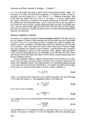
of our map, the expected mean distance between nearest neighbors is

-1
s’2m (5.24)

where A is the area of the map and n is the number of points. You will recall that
A/n is the point density, A. The sampling variance of is given by

(5.25)

If we work out the constants.

0.06831 A
g; = (5.26)
n2
The standard error of the mean distance between nearest neighbors is the square
root of CT;
0.26136
4-
se = (5.27)
-
The distribution of 6 is normal provided n is greater than 6, so we can use the
simple z-test given in Chapter 2 to test the hypothesis that the observed mean

310