Page 226 - Statistics for Environmental Engineers

L1592_frame_C25.fm Page 228 Tuesday, December 18, 2001 2:45 PM

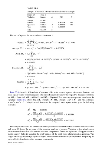
TABLE 25.4
Analysis of Variance Table for the Foundry Waste Example
Source of Sum of
Variation Squares df MS F
Average 0.10693 1
Batches 0.00367 2 0.001835 367
Specimens 0.00624 9 0.000693 139
Tests 0.00006 12 0.000005
Total 0.11690 24

The sum of squares for each variance component is:

n b n s n t
Total SS t ∑ ∑ ∑ y bst = 0.082 + 0.084 + … + 0.044 = 0.11690
=
2
2
2
b=1 s=1 t=1
(
Average SS ave = n b n s n t y = 34() 2() 0.06675) = 0.106934
2
2
n b
Batch SS b = n s n t∑ ( y b – y) 2
b=1
= 4 () 2() 0.0840 0.06675) +[ ( – 2 ( 0.0606 0.06675) + ( 0.0556 0.06675) ]
2
2
–
–
= 0.003671
n b n s
Specimen SS s = n t ∑∑ ( y bs – y b ) 2
b=1 s=1
= 2 0.083 0.0840) +[ ( – 2 ( 0.1085 0.0840) + … + ( 0.047 0.0556) ]
2
2
–
–
= 0.000624
n b n s n t
Test SS t ∑ ∑ ∑ ( y bst – y bs ) 2
=
b=1 s=1 t=1
2
2
2
= ( 0.082 0.083) + ( 0.084 0.083) + … + ( 0.044 0.0470) = 0.000057
–
–
–
Table 25.4 gives the full analysis of variance table, with sums of squares, degrees of freedom, and
mean square values. The mean squares (the sums of squares divided by the respective degrees of freedom)
are MS b = 0.001835, MS s = 0.000693, and MS t = 0.000005. The mean squares are used to estimate the
2
2 MS s estimates n t σ s + 2
variances. Table 25.3 shows that MS t estimates σ t , σ t , and MS b estimates
n s n t σ b + σ s + σ t . Using these relations with the computed mean square values gives the following
2
2
2
n t
estimates:
σ ˆ t = MS t = 0.000005
2
–
--------------------------------------------------- =
-------------------------- =
σ ˆ s = MS s – MS t 0.000693 0.000005 0.000344
2
n t 2
–
-------------------------- =
--------------------------------------------------- =
σ ˆ b = MS b – MS s 0.001836 0.000693 0.000143
2
n s n t 4 × 2
The analysis shows that the variance between specimens is about twice the variance of between batches
and about 60 times the variance of the chemical analysis of copper. Variation in the actual copper
measurements is small relative to other variance components. Extensive replication of copper measure-
ments scarcely helps in reducing the total variance of the solid waste characterization program. This
suggests making only enough replicate copper measurements to maintain quality control and putting the
major effort into reducing other variance components.
© 2002 By CRC Press LLC