Page 225 - Statistics for Environmental Engineers

L1592_frame_C25.fm Page 227 Tuesday, December 18, 2001 2:45 PM

TABLE 25.3
General Analysis of Variance Table for Estimating the Variance Components from a Three-Factor Nested
Experimental Design
Source of Degrees of Mean Square
Variation Sum of Squares Freedom Mean Square Estimates
2
Average SS ave = n b n s n t y 1
(
n b 2 SS b 2 2 2
Batches SS b = n s n t ∑ b=1 y b – y) n b − 1 MS b = ------------- n s n t σ b + n t σ s + σ t
n b – 1
(
n b n s 2 SS s 2 2
Specimens SS s = n t ∑ b=1 ∑ s=1 y bs – y s ) n b (n s − 1) MS s = ----------------------- n t σ s + σ t
(
n b n s – 1)
(
n b n s n t 2 SS t 2
Tests SS t = ∑ b=1 ∑ s=1 ∑ t=1 y bst – y bs ) n b n s (n t − 1) MS t = ---------------------------- σ t
(
n b n s n t – 1)
n b n s n t 2
Total SS T = ∑ b=1 ∑ s=1 ∑ t=1 y bst
Variation in tests
performed on the
same specimen
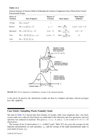
σ t y obs = η + e t + e s + e b
t e
Overall mean t s b Variation in
e + e + e
specimens obtained
from the same batch
e
s σ s
e + e b
s
Variation due to
nonhomogeneity
σ b between batches

y
e
Overall mean = η b η + e
b
FIGURE 25.3 Error components contributing to variance in the measured quantity.

is also given. In practice, the calculations usually are done by computer and many software packages
have this capability.

Case Study: Sampling Waste Foundry Sand

The data in Table 25.2 showed that three batches of foundry solid waste (baghouse dust, core butts,
system sand) were collected. Each batch was subdivided in the laboratory into four specimens, and each
specimen was analyzed in duplicate. This gives n b = 3, n s = 4, and n t = 2, for a total of 3 × 4 × 2 = 24
observations.
The average of the 24 observations is = 0.06673 mg/L. Table 25.2 also gives the averages for the
y
duplicate measurements on each specimen, y bs , and the average of the eight measurements made on
each batch of waste (y b ).
© 2002 By CRC Press LLC