Page 227 - Statistics for Environmental Engineers

L1592_frame_C25.fm Page 229 Tuesday, December 18, 2001 2:45 PM

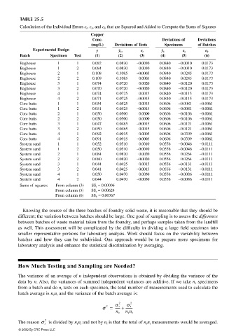
TABLE 25.5
Calculation of the Individual Errors e t , e s , and e b that are Squared and Added to Compute the Sums of Squares
Copper
Conc. Deviations of Deviations
(mg/L) Deviations of Tests Specimens of Batches
Experimental Design y y bs e t y b e s e b
Batch Specimen Test (1) (2) (3) (4) (5) (6)
Baghouse 1 1 0.082 0.0830 −0.0010 0.0840 −0.0010 0.0173
Baghouse 1 2 0.084 0.0830 0.0010 0.0840 −0.0010 0.0173
Baghouse 2 1 0.108 0.1085 −0.0005 0.0840 0.0245 0.0173
Baghouse 2 2 0.109 0.1085 0.0005 0.0840 0.0245 0.0173
Baghouse 3 1 0.074 0.0720 0.0020 0.0840 −0.0120 0.0173
Baghouse 3 2 0.070 0.0720 −0.0020 0.0840 −0.0120 0.0173
Baghouse 4 1 0.074 0.0725 0.0015 0.0840 −0.0115 0.0173
Baghouse 4 2 0.071 0.0725 −0.0015 0.0840 −0.0115 0.0173
Core butts 1 1 0.054 0.0525 0.0015 0.0606 −0.0081 −0.0061
Core butts 1 2 0.051 0.0525 −0.0015 0.0606 −0.0081 −0.0061
Core butts 2 1 0.050 0.0500 0.0000 0.0606 −0.0106 −0.0061
Core butts 2 2 0.050 0.0500 0.0000 0.0606 −0.0106 −0.0061
Core butts 3 1 0.047 0.0485 −0.0015 0.0606 −0.0121 −0.0061
Core butts 3 2 0.050 0.0485 0.0015 0.0606 −0.0121 −0.0061
Core butts 4 1 0.092 0.0915 0.0005 0.0606 0.0309 −0.0061
Core butts 4 2 0.091 0.0915 −0.0005 0.0606 0.0309 −0.0061
System sand 1 1 0.052 0.0510 0.0010 0.0556 −0.0046 −0.0111
System sand 1 2 0.050 0.0510 −0.0010 0.0556 −0.0046 −0.0111
System sand 2 1 0.084 0.0820 0.0020 0.0556 0.0264 −0.0111
System sand 2 2 0.080 0.0820 −0.0020 0.0556 0.0264 −0.0111
System sand 3 1 0.044 0.0425 0.0015 0.0556 −0.0131 −0.0111
System sand 3 2 0.041 0.0425 −0.0015 0.0556 −0.0131 −0.0111
System sand 4 1 0.050 0.0470 0.0030 0.0556 −0.0086 −0.0111
System sand 4 2 0.044 0.0470 −0.0030 0.0556 −0.0086 −0.0111
Sums of squares: From column (3) SS t = 0.00006
From column (5) SS s = 0.00624
From column (6) SS b = 0.00367
‘

Knowing the source of the three batches of foundry solid waste, it is reasonable that they should be
different; the variation between batches should be large. One goal of sampling is to assess the difference
between batches of waste material taken from the foundry, and perhaps samples taken from the landfill
as well. This assessment will be complicated by the difficulty in dividing a large field specimen into
smaller representative portions for laboratory analysis. Work should focus on the variability between
batches and how they can be subdivided. One approach would be to prepare more specimens for
laboratory analysis and enhance the statistical discrimination by averaging.

How Much Testing and Sampling are Needed?

The variance of an average of n independent observations is obtained by dividing the variance of the
data by n. Also, the variances of summed independent variances are additive. If we take n s specimens
from a batch and do n t tests on each specimen, the total number of measurements used to calculate the
batch average is n s n t and the variance of the batch average is:

2 2
σ = ------ + ---------
2
σ s
σ t
n s n s n t
2
The reason σ t is divided by n s n t and not by n t is that the total of n s n t measurements would be averaged.
© 2002 By CRC Press LLC