Page 224 - Statistics for Environmental Engineers

L1592_frame_C25.fm Page 226 Tuesday, December 18, 2001 2:45 PM

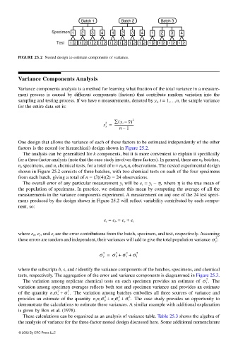
Batch 1 Batch 2 Batch 3
Specimen 1 2 3 4 1 2 3 4 1 2 3 4

Test 12 12 12 12 12 12 12 12 12 12 12 12

FIGURE 25.2 Nested design to estimate components of variance.

Variance Components Analysis
Variance components analysis is a method for learning what fraction of the total variance in a measure-
ment process is caused by different components (factors) that contribute random variation into the
sampling and testing process. If we have n measurements, denoted by y i , i = 1,…,n, the sample variance
for the entire data set is:

(
s y = ∑ y i – y) 2
2
------------------------
–
n 1
One design that allows the variance of each of these factors to be estimated independently of the other
factors is the nested (or hierarchical) design shown in Figure 25.2.
The analysis can be generalized for k components, but it is more convenient to explain it specifically
for a three-factor analysis (note that the case study involves three factors). In general, there are n b batches,
n s specimens, and n t chemical tests, for a total of n = n b n s n t observations. The nested experimental design
shown in Figure 25.2 consists of three batches, with two chemical tests on each of the four specimens
from each batch, giving a total of n = (3)(4)(2) = 24 observations.
The overall error of any particular measurement y i will be e i = y i − η, where η is the true mean of
the population of specimens. In practice, we estimate this mean by computing the average of all the
measurements in the variance components experiment. A measurement on any one of the 24 test speci-
mens produced by the design shown in Figure 25.2 will reflect variability contributed by each compo-
nent, so:

e i = e b + e s + e t

where e b , e s , and e t are the error contributions from the batch, specimen, and test, respectively. Assuming
2
these errors are random and independent, their variances will add to give the total population variance σ y :

σ y = σ b + σ s + σ t 2
2
2
2
where the subscripts b, s, and t identify the variance components of the batches, specimens, and chemical
tests, respectively. The aggregation of the error and variance components is diagrammed in Figure 25.3.
2
The variation among replicate chemical tests on each specimen provides an estimate of σ t . The
variation among specimen averages reflects both test and specimen variance and provides an estimate
2
of the quantity n t σ s + σ t . The variation among batches embodies all three sources of variance and
2
provides an estimate of the quantity n s n t σ b + σ s + σ t . The case study provides an opportunity to
2
2
2
n t
demonstrate the calculations to estimate these variances. A similar example with additional explanation
is given by Box et al. (1978).
These calculations can be organized as an analysis of variance table. Table 25.3 shows the algebra of
the analysis of variance for the three-factor nested design discussed here. Some additional nomenclature
© 2002 By CRC Press LLC