Page 164 - Sustainability in the Process Industry Integration and Optimization

Fu r t h e r A p p l i c a t i o n s o f P r o c e s s I n t e g r a t i o n 141

Step 3. Display the optimal biomass exchange fl ows. A visual mapping
of interzone biomass exchanges provides critical feedback for
the decision maker. The zone “centroids” are plotted in two-
dimensional Cartesian coordinates.
Step 4. Form the clusters. Mixed integer linear programming (MILP)
has proven to be a convenient tool for this task.
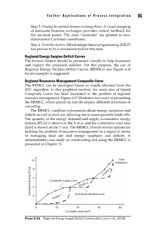
Regional Energy Surplus-Deficit Curves
The formed clusters should be presented visually to help document
and explain the proposed solution. For this purpose, the use of
Regional Energy Surplus-Deficit Curves (RESDCs) (see Figure 6.16
for an example) is suggested.
Regional Resources Management Composite Curve
The RRMCC can be developed based on results obtained from the
REC algorithm. In this graphical method, the main idea of Grand
Composite Curve has been translated to the problem of regional
resource management. Figure 6.17 illustrates two ways of presenting
the RRMCC, where panels (a) and (b) employ different directions of
cascading.
The RRMCC combines information about energy surpluses and
deficits as well as land use, allowing one to assess possible trade-offs.
The quantity of the energy demand and supply (cumulative energy
balance [PJ/y]) is shown on the X axis, and the cumulative zone area
2
[km ] is shown on the Y axis. The RRMCC reveals several options for
tackling the problem of resources management in a region in terms
of managing land use and energy surpluses and deficits. A
demonstration case study on constructing and using the RRMCC is
presented in Chapter 11.

10 Total
Imbalance
Cumulative Energy [PJ/y] 6 4 Cumulative supply curve Cluster 2 Cluster 3
8

Cluster 1 Cumulative demand curve
2

0 20 40 60 80
Cumulative Area [km ] 2
FIGURE 6.16 Regional Energy Supply-Defi cit Curves (after Lam et al., 2009).