Page 24 - The Geological Interpretation of Well Logs

- THE GEOLOGICAL INTERPRETATION OF WELL LOGS ~-

resistivity 2

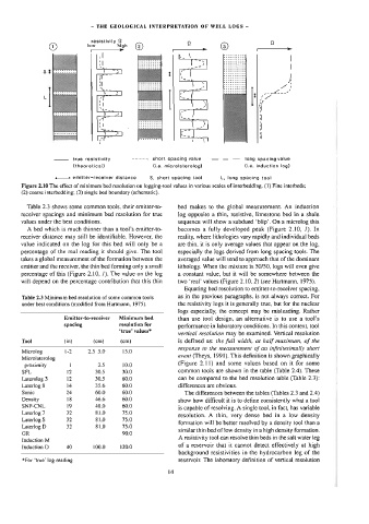
I ow hi gh (@)

-——

true resistivity short spacing valve long spacing value
(theoretical) (i.e. microlaterolog) (i.e. induction log)

ee emitter-receiver distance S, short spacing tool L, long spacing tool
Figure 2.10 The effect of minimum bed resolution on logging-tool values in various scales of interbedding. (1) Fine interbeds;
(2) coarse interbedding; (3) single bed boundary (schematic).

Table 2.3 shows some common tools, their emitter-1o- bed makes to the global measurement. An induction
receiver spacings and minimum bed resolution for true log opposite a thin, resistive, limestone bed in a shale
values under the best conditions. sequence wil] show a subdued ‘blip’. On a microlog this
A bed which is much thinner than a tool’s emitter-to- becomes a fully developed peak (Figure 2.10, 7). In
receiver distance may stil] be identifiable. However, the reality, where lithologies vary rapidly and individual beds
value indicated on the log for this bed will only be a are thin, it is only average values that appear on the log,
percentage of the real reading it should give. The tool especially the logs derived from long spacing tools. The
takes a global measurement of the formation between the averaged value will tend to approach that of the dominant
emitter and the receiver, the thin bed forming only a small lithology. When the mixture is 50/50, logs will even give
percentage of this (Figure 2.10, /). The value on the log a constant value, but it will be somewhere between the
will depend on the percentage contnbution that this thin two ‘real’ values (Figure 2.10, 2) (see Hartmann, 1975).
Equating bed resolution to emitter-to-receiver spacing,
Table 2.3 Minimum bed resolution of some common tools as in the previous paragraphs, is not always correct. For
under best conditions (modified from Hartmann, 1975). the resistivity logs it is generally true, but for the nuclear
logs especially, the concept may be misleading. Rather

Emitter-to-receiver Minimum bed than use tool design, an alternative is to use a tool’s
spacing resohution for performance in laboratory conditions, [n this context, tool
‘true’ values*
vertical resolution may be examined. Vertical resolution
Tool (in) (cm) (cm) is defined as: the full width, at half maximum, of the

response to the measurement of an infinitesimally short
Microlog 1-2 2.5 3.0 15.0
event (Theys, 1991). This definition is shown graphically
Microlaterolog
(Figure 2.11) and some values based on it for some
proximity l 2.5 10.0
SFL 12 30.5 30.0 common tools are shown in the table (Table 2.4). These
Laterolog 3 12 30.5 60.0 can be compared to the bed resolution table (Table 2.3):
Laterlog 8 14 35.6 60.0 differences are obvious.
Sonic 24 60.0 60.0 The differences between the tables (Tables 2.3 and 2.4)
Density 18 46.6 60.0 show how difficult it is to define consistently what a tool
SNP-CNL 19 48.0 60.0
is capable of resolving. A single tool, in fact, has variable
Laterlog 7 32 81.0 75.0
resolution. A thin, very dense bed in a low density
Laterlog S 32 81.0 75.0
formation will be better resolved by a density tool than a
Laterlog D 32 81.0 75.0
similar thin bed of low density in a high density formation.
GR 90.0
A resistivity tool can resolve thin beds in the salt water leg
Induction M
of a reservoir that it cannot detect effectively at high
Induction D 40 100.0 120.0
background resistivities in the hydrocarbon leg of the

*For ‘true’ log reading reservoir. The laboratory definition of vertical resolution