Page 73 - The Geological Interpretation of Well Logs

- RESISTIVITY AND CONDUCTIVITY LOGS -

“|
Deep Induction Qm?/m
LITH (generalised)
.
20.2
20
|.2
20.2
20|.2
.

—20).2 } 20].2 . 20.2 20 Locetion Map

9
f
@

d

c
eee ee
—,
?
b
a — vv 2 3 - S oN

8

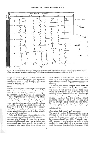
Figure 6.32 Correlation using deep induction logs (resistivity plots). The interval is one of thick, seemingly characterless, marine
shales. The togs show persistent, subtle changes which allow exceltent correlation over a distance of 30km.

changes in formation pressure and interstitial water sand with higher irreducible water will show lower
salinity which are non-stratigraphic, post-depositional resistivity. A clean, fining-upwards sandstone filted with
elements that tend to obliterate the original depositional hydrocarbons should show a regular upwards decrease in
features (cf. Figure 6.37). resistivity.
A second, well-known example, comes from the
Facies
Devonian of Canada (Figure 6.35; McCrossan, 1961).
From the shale example illustrated previously (Figure
The interval of study contains reefs and deeper water
6.31), it is clear that facies and facies changes can be
shales. The reefs contain oil. Careful mapping of the
followed on the resistivity logs. Indeed, it can be argued
resislivity values in the shales shows that a facies change
that a subtle lithological change is in fact a facies change.
occurs as the reefs are approached, reflected in an
One of the principal uses of the resistivity log in facies
increase in resistivity. The effect is probably one of
analysis is its ability to register changes in quartz (sand)-
increasing carbonate content and decreasing shale
shale mixtures. This is especially so in the fine-grained
porosity, although bedding characteristics also change.
rocks, shales and silts, more so than in sandstones them-
However, mapping the resistivity values enabled a more
selves. The example (Figure 6.33) shows small-scale
accurate localisation of the near-reef shale facies and the
deltaic cycles 15 m-20 m thick, picked out by resistivity
reefs themselves.
trends. The increase in resistivity corresponds to an
increase in the silt (quartz) content. Even slight, subcyclic Compaction, shale porosity and overpressure
events are visible on the logs. The normal compaction of shale seen along a borehole
Within sands themselves, it is suggested that in hydro- shows up in a plot of shale resistivity against depth: as
carbon-bearing zones, different resistivity values may be compaction increases so the resistivity increases (in a
correlated with differences in grain size. A coarser- homogeneous shale) (Figure 6.36). This trend is espe-
grained sand will genera]ly have a low irreducible water cially apparent in conductivities and a plot of shale
saturation and hence higher resistivity, the saturation in conductivity (deep induction) on a log scale against
hydrocarbons being higher (Figure 6.34). A fine-grained depth shows a near-linear distribution (Macgregor, 1965)

63