Page 340 - The Handbook for Quality Management a Complete Guide to Operational Excellence

326 C o n t i n u o u s I m p r o v e m e n t A n a l y z e S t a g e 327

25
Line
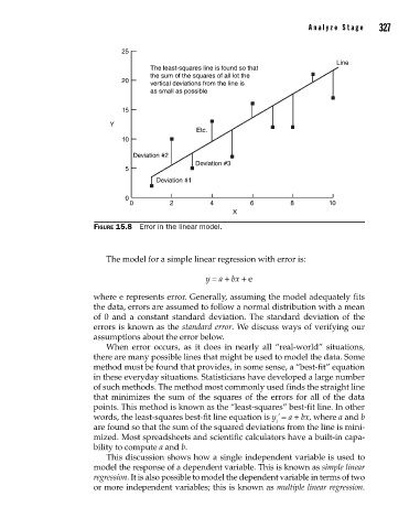
The least-squares line is found so that
the sum of the squares of all lot the
20 vertical deviations from the line is
as small as possible

15
Y
Etc.
10
Deviation #2
Deviation #3
5
Deviation #1

0
0 2 4 6 8 10
X
Figure 15.8 Error in the linear model.

The model for a simple linear regression with error is:

y = a + bx + e

where e represents error. Generally, assuming the model adequately fits
the data, errors are assumed to follow a normal distribution with a mean
of 0 and a constant standard deviation. The standard deviation of the
errors is known as the standard error. We discuss ways of verifying our
assumptions about the error below.
When error occurs, as it does in nearly all “real-world” situations,
there are many possible lines that might be used to model the data. Some
method must be found that provides, in some sense, a “best-fit” equation
in these everyday situations. Statisticians have developed a large number
of such meth ods. The method most commonly used finds the straight line
that minimizes the sum of the squares of the errors for all of the data
points. This method is known as the “least-squares” best-fit line. In other
words, the least-squares best-fit line equation is y ’ = a + bx, where a and b
i
are found so that the sum of the squared deviations from the line is mini-
mized. Most spreadsheets and scientific calculators have a built-in capa-
bility to compute a and b.
This discussion shows how a single independent variable is used to
model the response of a dependent variable. This is known as simple linear
regression. It is also possible to model the dependent variable in terms of two
or more independent variables; this is known as multiple linear regression.

15_Pyzdek_Ch15_p305-334.indd 327 11/20/12 10:33 PM