Page 1119 - The Mechatronics Handbook

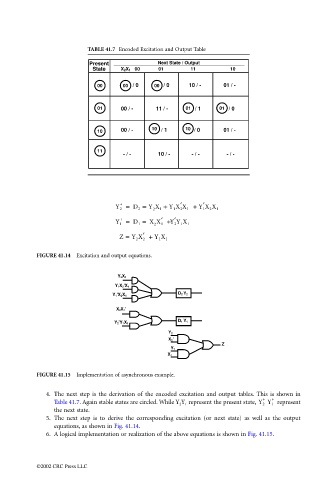
TABLE 41.7 Encoded Excitation and Output Table

Present Next State / Output
State X 2X 1 00 01 11 10

00 00 / 0 00 / 0 10 / - 01 / -

01 00 / - 11 / - 01 / 1 01 / 0

10 00 / - 10 / 1 10 / 0 01 / -

11
- / - 10 / - - / - - / -

+ ′ ′
Y 2 = D 2 = Y X 1 + Y 1 X 2 X 1 +
2 Y 1 X 2 X 1
+ ′ ′
Y 1 = D 1 = X X 1 + Y 2 Y 1 X 1
2
′
Z = Y 2 X 2 + Y 1 X 1

FIGURE 41.14 Excitation and output equations.

Y 2 X 1
Y 1 X 2 'X 1
D 2 Y 2
Y 1 'X 2 X 1
X 2 X 1 '
D 1 Y 1
Y 2 'Y 1 X 1
Y 2
X 2 '
Z
Y 1
X 1

FIGURE 41.15 Implementation of asynchronous example.

4. The next step is the derivation of the encoded excitation and output tables. This is shown in
+ +
Table 41.7. Again stable states are circled. While Y 2 Y 1 represent the present state, Y 2 Y 1 represent
the next state.
5. The next step is to derive the corresponding excitation (or next state) as well as the output
equations, as shown in Fig. 41.14.
6. A logical implementation or realization of the above equations is shown in Fig. 41.15.

©2002 CRC Press LLC