Page 1114 - The Mechatronics Handbook

S 1 (0,1)
(0,2)
(0,1)
S 2 (0,3) (0,2)
(0,3)
S 3
(0,1)
(0,2) (0,3)
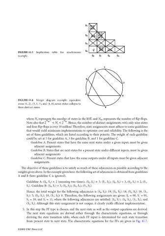
FIGURE 41.5 Implication table for synchronous S 4
example. S 0 S 1 S 2 S 3

1
7

6
2

5
3
FIGURE 41.6 Merger diagram example: equivalent
states (1, 2), (3, 5, 7), and (4, 6), seven states collapse to
three distinct states. 4

where N S represents the number of states in the RST, and N FF represents the number of flip-flops.
N -1 N
Note also that 2 FF < N s < 2 FF . Hence, the number of distinct assignments with only nine states
and four flip-flops is over 10 million! Therefore, state assignments must adhere to some guidelines
that would yield minimum implementations to optimize cost and reliability. The following is the
set of three guidelines, which are listed according to their priority. The weight of each guideline
could be set at 5 for guideline A, 3 for guideline B, and 1 for guideline C.
Guideline A. Present states that have the same next states under a given input, must be given
adjacent assignments.
Guideline B. States that are next states for a present state under different inputs, must be given
adjacent assignments
Guideline C. Present states that have the same outputs under all inputs must be given adjacent
assignments.

The objective of these guidelines is to satisfy as much of these adjacencies as possible according to the
weights given above. In the example given here, the following set of adjacencies is obtained from guidelines
A and B (here guideline C is ignored).

Guideline A: (S 0 , S 1 ) × 2 (meaning two times), (S 0 , S 2 ) × 3, (S 1 , S 2 ), (S 0 , S 3 ) × 3, (S 2 , S 3 ) × 2, (S 1 ,
S 3 ). Guideline B: (S 0 , S 1 ) × 3, (S 0 , S 2 ), (S 0 , S 3 ), (S 1 , S 3 ).
Hence, the total weight for the following adjacencies is (S 0 , S 1 ): 19, (S 0 , S 2 ): 18, (S 0 , S 3 ): 18, (S 1 ,
S 2 ): 5, (S 2 , S 3 ): 10, (S 1 , S 3 ): 8. Therefore, the following assignments are given: S 0 = 00, S 1 = 01,
S 2 = 10, and S 3 = 11, where the following adjacencies are satisfied: (S 0 , S 1 ), (S 0 , S 2 ), (S 1 , S 3 ), and
(S 2 , S 3 ). Although this state assignment is not unique, it clearly yields efficient implementation.
5. In this step the FF type is chosen, and the next state as well as the output equations are derived.

The next state equations are derived either through the characteristic equations, or through
deriving the state transition table, where each FF input is determined for each state transition
from present state to next state. The characteristic equations for the FFs are given in Fig. 41.7,

©2002 CRC Press LLC