Page 534 - The Mechatronics Handbook

0066_Frame_C20 Page 4 Wednesday, January 9, 2002 5:41 PM

B

H H

FIGURE 20.4 µ-H diagram and B-H diagram.

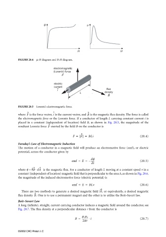
FIGURE 20.5 Lorentz’s electromagnetic force.

i
where is the force vector, is the current vector, and B is the magnetic flux density. The force is called
F
the electromagnetic force or the Lorentz force. If a conductor of length L carrying constant current i is
placed in a constant (independent of location) field B, as shown in Fig. 20.5, the magnitude of the
resultant Lorentz force exerted by the field B on the conductor is
F
F = |F| = BLi (20.4)

Faraday’s Law of Electromagnetic Induction
The motion of a conductor in a magnetic field will produce an electromotive force (emf), or electric
potential, across the conductor given by
dφ
emf = E = −------ (20.5)
dt
⋅
where φ = ∫ °B dA is the magnetic flux. For a conductor of length L moving at a constant speed v in a
constant (independent of location) magnetic field that is perpendicular to the area A, as shown in Fig. 20.6,
the magnitude of the induced electromotive force (electric potential) is

emf = E = BLv (20.6)
There are two methods to generate a desired magnetic field H , or equivalently, a desired magnetic
flux density . One is to use a permanent magnet and the other is to utilize the Boit–Savart law.
B
Boit–Savart Law
A long (infinite), straight, current carrying conductor induces a magnetic field around the conductor, see
Fig. 20.7. The flux density at a perpendicular distance r from the conductor is

B = ---------- i⋅ (20.7)
µ r µ 0
2πr

©2002 CRC Press LLC