Page 624 - The Mechatronics Handbook

0066_Frame_C20 Page 94 Wednesday, January 9, 2002 5:49 PM

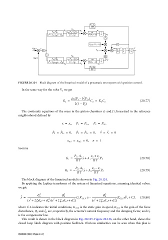
FIGURE 20.124 Block diagram of the linearized model of a pneumatic servosystem with position control.

In the same way for the valve V 2 we get
∗
(
r n P s – b 2 P 2r )
G 2 = ---------------------------------C 2 = K 2 C 2 (20.77)
∗
(
21 b 2 )
–
The continuity equations of the mass in the piston chambers e) and f ), linearized in the reference
neighborhood defined by
x = x r , P 1 = P 1r , P 2 = P 2r ,

P 1 = P 1r = 0, P 2 = P 2r = 0, x ˙ = x ˙ r = 0
˙
˙
˙
˙
x m1 = x m2 = 0, n = 1
become
x 0 +
G 1 = P 1r A 1 + ---------------P 1 (20.78)
x r
˙
-------------x ˙ A 1
RT RT
G 2 = −-------------x ˙ A 2 x 0 – x r ˙ (20.79)
+
P 2r A 2
---------------P 2
RT RT
The block diagram of the linearized model is shown in Fig. 20.124.
By applying the Laplace transforms of the system of linearized equations, assuming identical valves,
we get:
2 2 2
x ˙ = --------------------------------------------------------------------------------------G c K OLV e – ---------------------------------------------K OLF sF e + C.I. (20.80)
s A
s A
s n
2
( s + 2zs n s + s n ) s + 2z A s A s + s A ) ( s + 2z A s A s + s A )
2
2
2
2
(
2
where C.I. indicates the initial conditions, K OLV is the static gain in speed, K OLF is the gain of the force
disturbance, σ A and ζ A are, respectively, the actuator’s natural frequency and the damping factor, and G c
is the compensator law.
This result is shown in the block diagram in Fig. 20.125. Figure 20.126, on the other hand, shows the
closed loop block diagram with position feedback. Obvious similarities can be seen when this plan is
©2002 CRC Press LLC