Page 654 - The Mechatronics Handbook

0066_Frame_C20.fm Page 124 Wednesday, January 9, 2002 1:47 PM

T
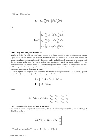
Using r = T r r , one has
2
B ei = B i + --------T r r + 1 T ∂ B i T
∂B i
T
----------T r r
--r T r
∂r 2 ∂r 2
and
2
-------T r r +
B x + ∂B x T 1 T ∂ B x T
---------T r r
--r T r
∂r 2 ∂ r 2
2
-------T r r +
B e = T r B y + ∂B y T 1 T ∂ B y T
---------T r r
--r T r
∂r 2 ∂ r 2
2
∂B ∂ B
z
B z + -------T r r + 1 T ---------T r r
T
z
T
--r T r
∂ r 2 ∂ r 2
Electromagnetic Torques and Forces
Now let us derive the fields and gradients at any point in the permanent magnet using the second-order
Taylor series approximation. To eliminate the transformations between the inertial and permanent
magnet coordinate systems and simplify the second-order negligible small components, we assume that
the relative motion between the magnet and the reference inertial coordinate is zero and the T rs trans-
formation matrix is used (otherwise, the second-order gradient terms will lead to cumbersome results).
The magnetization (the magnetic moment per unit volume) is constant over the volume of the
permanent-magnet thin films, and m = Mv.
Assuming that the magnetic flux is constant, the total electromagnetic torque and force on a planar
current loop (microwinding) in the uniform magnetic field is
T = ∫ ( M × B e + × ( M ∇)B e ) v
⋅
d
r
v
⋅
F = ∫ ( M ∇)B e v
d
v
where
M x
B exx B exy B exz
⋅
( M ∇)B e = [ ∂B e ]M = B eyx B eyy B eyz M y
B ezx B ezy B ezz M z

Case 1: Magnetization Along the Axis of Symmetry
For orientation of the magnetization vector along the axis of symmetry (x-axis) of the permanent-magnet
thin films, we have

B exx
⋅
( M ∇)B e = [ ∂B e ]M = M B exy
x
B exz
⋅
Thus, in the expression T = ∫ v (M × B e + r × (M ∇)B e )d , v

©2002 CRC Press LLC