Page 708 - Bird R.B. Transport phenomena

688 Chapter 22 Interphase Transport in Nonisothermal Mixtures

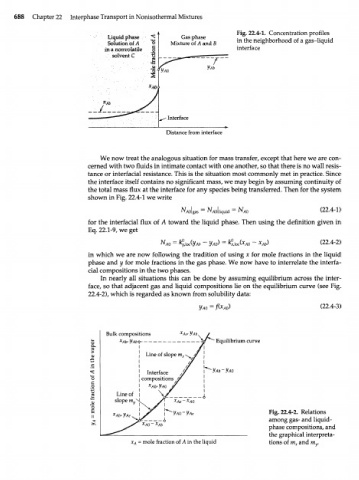
Fig. 22.4-1. Concentration profiles
Liquid phase Gas phase
Solution of A Mixture of A and В in the neighborhood of a gas-liquid
in a nonvolatile interface
solvent С

Distance from interface

We now treat the analogous situation for mass transfer, except that here we are con-
cerned with two fluids in intimate contact with one another, so that there is no wall resis-
tance or interfacial resistance. This is the situation most commonly met in practice. Since
the interface itself contains no significant mass, we may begin by assuming continuity of
the total mass flux at the interface for any species being transferred. Then for the system
shown in Fig. 22.4-1 we write
tyjgas = illiquid = Мдо (22.4-1)
for the interfacial flux of A toward the liquid phase. Then using the definition given in
Eq. 22.1-9, we get
~~ x Ab) (22.4-2)
in which we are now following the tradition of using x for mole fractions in the liquid
phase and у for mole fractions in the gas phase. We now have to interrelate the interfa-
cial compositions in the two phases.
In nearly all situations this can be done by assuming equilibrium across the inter-
face, so that adjacent gas and liquid compositions lie on the equilibrium curve (see Fig.
22.4-2), which is regarded as known from solubility data:

(22.4-3)
У АО =

Bulk compositions Х АСУАЬ
*f Equilibrium <
7
XAI-ШЖ I/ A h f*
Line of slope m v^ //
x
//
//
Interface /f ^УАЬ-УАО
compositions у
x
A0^A0 /
Line of
x
slope m \L A~ x Ae~ A0
y
х Fig. 22.4-2. Relations
АЫУАе \S 1
among gas- and liquid-
x
^ ^ x A0 ~ Ab phase compositions, and
the graphical interpreta-
x A = mole fraction of A in the liquid tions of m and m r
x