Page 61 - Using ANSYS for Finite Element Analysis A Tutorial for Engineers

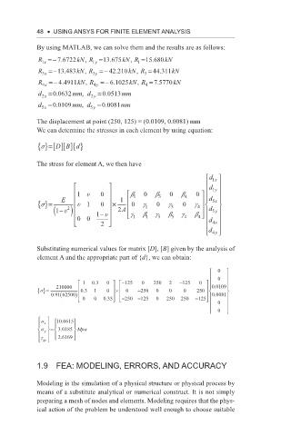
48 • Using ansys for finite element analysis
By using MATLAB, we can solve them and the results are as follows:

.
,
.
R =− . kNR = 13 675 kN R = 15 680 kN
,
7 6722
x 1 1 y 1
R =− 13 483 kNR =−, 42 210. kN , R = 44 311kN
.
2
.
3 x 3 y 3
R =− 4 4911kNR 4y =− 6 1025kN R = 7 5770kN
N
.
,
.
,
.
4x
4
d 2 x = 0 0632 mmd 2 y = 0 0513 mm
.
,
.
d = 0 0109 mmd = 0 0081 mm
.
,
.
5 x 5 y
The displacement at point (250, 125) = (0.0109, 0.0081) mm
We can determine the stresses in each element by using equation:
s {}=[][]{}
DB d
The stress for element A, we then have
d 1 
x
   d 1y 
1 u 0  b  0 b 0 b 0   


E   1  1 5 4   d 5x 

s {}=  u 1 0  ×  0 g 1 0 g 5 0 g 4 4  

2
− ( 1 u )   2 A  d 5y 
1 − u  g  b g b g b 
4 
00  1 1 5 5 4  d 
 2   4x 
 d 4y 


Substituting numerical values for matrix [D], [B] given by the analysis of
element A and the appropriate part of {d}, we can obtain:
 0 
 0 
 1 0 3 0   −125 0 250 2 −1125 0    0 0109 
.

×
s {}= 210000  03 1 0   0 − 250 0 0 0 250  . 
.
.
091 (62500 )      0 0081 1 
.
  0 0 035   − 250 − 125 0 250 250 − 125    
 
.
 0 
 0 
 s   10 0615
.
  x    
 s y  =  3 0185  Mpa
.
 t   2..6169  
  xy   
1.9 fea: modeling, errors, and aCCUraCy
Modeling is the simulation of a physical structure or physical process by
means of a substitute analytical or numerical construct. It is not simply
preparing a mesh of nodes and elements. Modeling requires that the phys-
ical action of the problem be understood well enough to choose suitable