Page 111 - Water Engineering Hydraulics, Distribution and Treatment

89
4.2 Design Population
If it is assumed that the initial value of k, namely k ,
0
than remaining constant, k can be assigned the following
(L – y˝)
Growth curve
value:
e
(4.5)
k = k ∕(1 + nk t)
0
0
Population, y
b
in which n, as a coefficient of retardance, adds a useful con-
Point of inflection
y˝
cept to Eqs. (4.2)–(4.4).
Maximum
On integrating Eqs. (4.1)–(4.4) between the limits y = y
Rate of growth =
d
0
rate
at t = 0 and y = y at t = t for unchanging k values, they
change as shown next.
For autocatalytic first-order progression (arc ac in
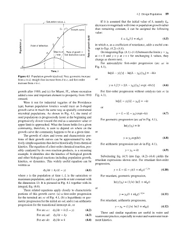
y´ Saturation value, L first derivative curve c Rate of growth dy/dt decreases in magnitude with time or population growth rather
a Fig. 4.1),
Time, t
ln[(L − y)∕y] −ln[(L − y )∕y ] =−kLt
0
0
Figure 4.1 Population growth idealized. Note geometric increase
from a to d, straight-line increase from d to e, and first-order or
increase from e to c.
y = L∕{1 + [(L − y )∕y ] exp(−kLt)} (4.6)
0
0
growth after 1910; and (c) for Miami, FL, where recreation For first-order progression without catalysis (arc ec in
added a new and important element to prosperity from 1910 Fig. 4.1),
onward.
ln[(L − y)∕(L − y )] =−kt
Were it not for industrial vagaries of the Providence 0
type, human population kinetics would trace an S-shaped or
growth curve in much the same way as spatially constrained
microbial populations. As shown in Fig. 4.1, the trend of y = L − (L − y ) exp(−kt) (4.7)
0
seed populations is progressively faster at the beginning and
For geometric progression (arc ad in Fig. 4.1),
progressively slower toward the end as a saturation value or
upper limit is approached. What the future holds for a given ln(y∕y ) = kt
0
community, therefore, is seen to depend on where on the
growth curve the community happens to be at a given time. or
The growth of cities and towns and characteristic por-
y = y exp(kt) (4.8)
tions of their growth curves can be approximated by rela- 0
tively simple equations that derive historically from chemical
For arithmetic progression (arc de in Fig. 4.1),
kinetics. The equation of a first-order chemical reaction, pos-
sibly catalyzed by its own reaction products, is a recurring y − y = kt (4.9)
0
example. It identifies also the kinetics of biological growth
Substituting Eq. (4.5) into Eqs. (4.2)–(4.4) yields the
and other biological reactions including population growth,
retardant expressions shown next. For retardant first-order
kinetics, or dynamics. This widely useful equation can be
progression,
written as
dy∕dt = ky (L − y) (4.1) y = L − (L − y)(1 + nk t) −1∕n (4.10)
0
where y is the population at time t, L is the saturation or For retardant, geometric progression,
maximum population, and k is a growth or rate constant with
the dimension 1/t. It is pictured in Fig. 4.1 together with its ln(y∕y ) = (1∕n) ln(1 + nk t)
0
0
integral, Eq. (4.6).
or
Three related equations apply closely to characteristic
portions of this growth curve: (a) a first-order progression y = y (1 + nk t) −1∕n (4.11)
0
0
for the terminal arc ec of Fig. 4.1, (b) a logarithmic or geo-
metric progression for the initial arc ad, and (c) an arithmetic For retardant, arithmetic progression,
progression for the transitional intercept de,or
y − y = (1∕n) ln(1 + nk t) (4.12)
0
0
For arc ec: dy∕dt = k (L − y) (4.2)
These and similar equations are useful in water and
For arc ad: dy∕dt = ky (4.3)
wastewater practice, especially in water and wastewater treat-
For arc de: dy∕dt = k (4.4) ment kinetics.