Page 113 - Water Engineering Hydraulics, Distribution and Treatment

(a) Arithmetic
1960
log y = 5.4654
y = 292,000
j
j
log y = 5.3962
1950
y = 249,000
i
i
y − y = 43,000
log y −log y = 0.0692
j
j
i
0.925(log y −log y ) = 0.0620
0.925(y − y ) = 40,000
i
j
j
1969
y = 332,000
y = 337,000
m
m
Geometric estimates are seen to be lower than arithmetic estimates for intercensal years and higher for postcensal years.
The US Bureau of the Census estimates the current pop- or (b) Geometric i i 4.2 Design Population 91
ulation of the whole nation by adding to the last census pop-
y = L∕[1 + p exp( − qt)]
ulation the intervening differences (a) between births and
deaths, that is, the natural increases; and (b) between immi- y = L∕[1 +exp(ln p − qt)]
gration and emigration. For states and other large population
groups, postcensal estimates can be based on the apportion- and equating the first derivative of Eq. (4.1) to zero, or
ment method, which postulates that local increases will equal
d(dy∕dt)∕dt = kL − 2ky = 0
the national increase times the ratio of the local to the national
intercensal population increase. Intercensal losses in popu- It follows that the maximum rate of growth dy∕dt is
lation are normally disregarded in postcensal estimates; the obtained when
last census figures are used instead.
Supporting data for short-term estimates can be derived y = 1∕2L
from sources that reflect population growth in ways differ-
and
ent from, yet related to, population enumeration. Examples
are records of school enrollments; house connections for t = (−ln p)∕q = (−2.303 log p)∕q
water, electricity, gas, and telephones; commercial trans-
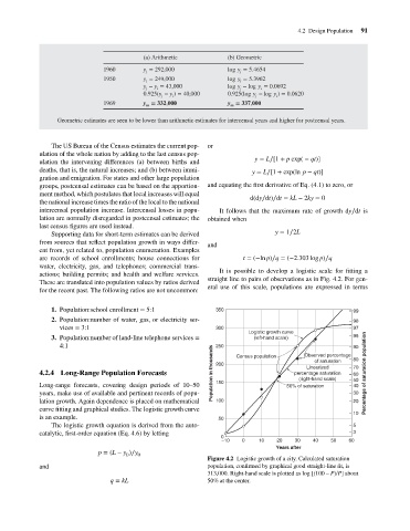
It is possible to develop a logistic scale for fitting a
actions; building permits; and health and welfare services.
straight line to pairs of observations as in Fig. 4.2. For gen-
These are translated into population values by ratios derived
eral use of this scale, populations are expressed in terms
for the recent past. The following ratios are not uncommon:
1. Population:school enrollment = 5:1 350 99
2. Population:number of water, gas, or electricity ser- 98
vices = 3:1 300 97
Logistic growth curve
3. Population:number of land-line telephone services = (left-hand scale) 95
4:1 250 Census population Observed percentage 90
Population in thousands (right-hand scale) 60 Percentage of saturation population
of saturation
Linearized
70
4.2.4 Long-Range Population Forecasts 200 percentage saturation 80
Long-range forecasts, covering design periods of 10–50 150 50% of saturation 50
40
years, make use of available and pertinent records of popu- 30
lation growth. Again dependence is placed on mathematical 100 20
curve fitting and graphical studies. The logistic growth curve
10
is an example. 50
The logistic growth equation is derived from the auto- 5
catalytic, first-order equation (Eq. 4.6) by letting 3
0
–10 0 10 20 30 40 50 60
Years after
p = (L − y )∕y
0 0
Figure 4.2 Logistic growth of a city. Calculated saturation
and population, confirmed by graphical good straight-line fit, is
313,000. Right-hand scale is plotted as log [(100 – P)/P] about
q = kL 50% at the center.