Page 193 - Characterization and Properties of Petroleum Fractions - M.R. Riazi

QC: —/—
P2: KVU/KXT
P1: KVU/KXT
AT029-Manual
AT029-Manual-v7.cls
21:30
June 22, 2007
AT029-04
300
800
0.9
Actual Data for Tb
Actual data T1: IML 4. CHARACTERIZATION OF RESERVOIR FLUIDS AND CRUDE OILS 173
Predicted Tb
Optimum B 600 Actual data for SG
Molecular Weight, M 100 Boiling Point, T b , K 400 0.8 Specific Gravity, SG
B=1
Predicted SG
200
200
0 0 0.7
0 0.2 0.4 0.6 0.8 1
0 0.2 0.4 0.6 0.8 1
Cumulative Mole Fraction, x cm Cumulative Weight Fraction, x cm
FIG. 4.11—Prediction of molar distribution from FIG. 4.12—Prediction of boiling point and specific gravity dis-
Eq. (4.56) for the GC system of Example 4.7. tributions from Eq. (4.56) for the GC system of Example 4.7.

If the fixed value of B M = 1 is used with M o = 89.86 and
A M = 0.3105 then the molar distribution is given by a sim-
pler relation
1

M = 89.86 1 + 0.3105 ln -1
1 − x cm
Prediction of molar distribution based on these two relations Data
(B M = 0.9429 and B M = 1) are shown in Fig. 4.11. The two Predicted
curves are almost identical except toward the end of the curve
where x cm → 1 and the difference is not visible in the figure.
Using a similar approach, coefficients in Eq. (4.56) for T b Y = ln SG *
and SG are determined. For SG both cumulative weight and
volume fractions can be used. The value of T b for the residue -2
(C 18+ ) is not known, for this reason only 11 data points
are used for the regression analysis. Summary of results
for coefficients of Eq. (4.56) for M, T b , and SG in terms of
various x c is given in Table 4.13. Based on these coefficients
T b and SG distributions predicted from Eq. (4.56) are shown
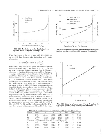
in Fig. 4.12. The linear relation between parameters X and Y
defined in Eq. (4.57) for SG is demonstrated in Fig. 4.13. Pre-
diction of PDF for T b and SG are shown in Figs. 4.14 and 4.15,
respectively. Both Eqs. (4.66) and (4.70) have been used to -3
illustrate density function for both T b and SG. As shown in -2 -1 0 1 2
Table 4.13, the best values of M o , T bo , and SG o are 91, 350 K,
and 0.705, which are very close to the values of lower bound- X = ln ln (1/x*)
ary properties for the C 7+ group. (M = 88, T b7 = 350 K,
−
−
7
SG = 0.709). For GC and light oils values of B for M are FIG. 4.13—Linearity of parameters Y and X defined in
−
7
very close to one, for T b are close to 1.5, and for SG are close Eq. (4.57) for specific gravity of the system in Example 4.7.
TABLE 4.13—Coefficients of Eq. (4.56) for M, T b , and SG for data of Table 4.11.
Property Type of x c P o A B RMS %AAD R 2
M Mole 91 0.2854 0.9429 2.139 0.99 0.999
Weight 350 (K) 0.1679 1.2586 3.794 0.62 0.998
T b
SG Volume 0.705 0.0232 1.8110 0.004 0.32 0.997
SG Weight 0.705 0.0235 1.8248 0.004 0.33 0.997
Coefficients of P o and A with fixed value of B for each property
M Mole 89.86 0.3105 1 2.83 1.39 0.998
T b Weight 340 (K) 0.1875 1.5 5.834 1.15 0.993
SG Volume 0.665 0.0132 3 0.005 0.54 0.984
SG Weight 0.6661 0.0132 3 0.005 0.53 0.985
--`,```,`,``````,`,````,```,,-`-`,,`,,`,`,,`---

Copyright ASTM International
Provided by IHS Markit under license with ASTM Licensee=International Dealers Demo/2222333001, User=Anggiansah, Erick
No reproduction or networking permitted without license from IHS Not for Resale, 08/26/2021 21:56:35 MDT