Page 191 - Characterization and Properties of Petroleum Fractions - M.R. Riazi

T1: IML
P2: KVU/KXT
P1: KVU/KXT
QC: —/—
AT029-Manual-v7.cls
June 22, 2007
21:30
AT029-04
AT029-Manual
4. CHARACTERIZATION OF RESERVOIR FLUIDS AND CRUDE OILS 171
mixture contains all compounds including extremely heavy
property P for C 7 or C 6 hydrocarbon group from Table 4.6
compounds up to M →∞. However, what differs from one for the value P o is always needed. For a C 7+ fraction value of
mixture to another is the amount of individual components. may be used as the initial guess. Although linear regression
For low and medium molecular weight range fractions that can be performed with spreadsheets such as Excel or Lotus,
do not contain high molecular weight compounds, the model coefficients C 1 and C 2 in Eq. (4.57) can be determined by hand
expressed by Eq. (4.56) assumes that extremely heavy com- calculators using the following relation derived from the least
pounds do exist in the mixture but their amount is infinitely squares linear regression method:
small, which in mathematical calculations do not affect mix- Y i − N (X i Y i )
ture properties. C 2 = X i 2 2

When sufficient data on property P versus cumulative mole, (4.60) ( X i) − N X i
weight, or volume fraction, x c , are available constants in Y i − C 2 X i
Eq. (4.56) can be easily determined by converting the equa- C 1 = N
tion into the following linear form:
where each sum applies to all data points used in the regres-
(4.57) Y = C 1 + C 2 X sion and N is the total number of points used. The least
squares linear regression method is a standard method for
where Y = ln P ∗ and X = ln[ln(1/x )]. By combining obtaining the equation of a straight line, such as Eq. (4.57),
∗
Eqs. (4.56) and (4.57) we have from a set of data on X i and Y i .
1
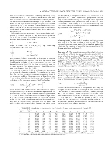
B = Example 4.7—The normalized composition of a C 7+ fraction
(4.58) C 2
derived from a North Sea gas condensate sample (GC) in
A = B exp(C 1 B)
terms of weight fractions of SCN groups up to C 17 is given
--`,```,`,``````,`,````,```,,-`-`,,`,,`,`,,`---
It is recommended that for samples with amount of residues in Table 4.11. M and SG of C 18+ fraction are 264 and 0.857,
(last hydrocarbon group) greater than 30%, the residue data respectively. For the whole C 7+ fraction the M 7+ and SG 7+ are
should not be included in the regression analysis to obtain 118.9 and 0.7597, respectively. Obtain parameters P o , A, and
the coefficients in Eq. (4.57). If a fixed value of B is used for B in Eq. (4.56) for M, T b , and SG and compare calculated
a certain property, then only parameter C 1 should be used to values of these properties with data shown in Table 4.6.
obtain coefficient A from Eq. (4.58).
To estimate P o in Eq. (4.56), a trial-and-error procedure Solution—For SCN groups from C 7 to C 17 values of M, T b , and
can be used. By choosing a value for P o , which must be lower SG can be taken from Table 4.6 and are given in Table 4.11.
than the first data point in the dataset, parameters A and B An alternative to this table would be values recommended by
can be determined from liner regression of data. Parameter Whitson [15] for SCN groups less than C 25 . Discrete mole frac-
P o can be determined by minimizing the error function E(P o ) tions, x mi can be calculated from discrete weight fractions, x wi
equivalent to the root mean squares (RMS) defined as and M i by a reversed form of Eq. (1.15) as follows:
1/2 x wi /M i
N (4.61)
1 exp 2 x mi = N
(4.59) E(P ◦ ) = P i calc − P i i=1 x wi /M i

N
i=1
where N is the total number of components (including the
where N is the total number of data point used in the regres- last plus fraction) and for this example it is 12. Discrete vol-
sion process and P i calc is the calculated value of property P for ume fractions x vi can be calculated from x wi and SG i through
the subfraction i from Eq. (4.56) using estimated parameters Eq. (1.16). Values of x mi and x vi are given in Table 4.11. To ob-
P o , A, and B. As an alternative objective function, best value tain parameters in Eq. (4.56), cumulative mole (x cm ), weight
of P o can be obtained by maximizing the value of R defined (x cw ), or volume (x cv ) fractions are needed. A sample calcu-
2
by Eq. (2.136). With spreadsheets such as Microsoft Excel, lation for the estimation of molecular weight versus x cm is
parameter P o can be directly estimated from the Solver tool shown here. A similar approach can be taken to estimate cu-
without trial-and-error procedure. However, an initial guess mulative weight or volume fractions.
TABLE 4.11—Sample data on characteristics of a C 7+ fraction for a gas condensate system in Example 4.7.
Fraction Carbon
No. No. x w M T b ,K SG x m x v x cm x cw x cv
1 7 0.261 95 365 0.727 0.321 0.273 0.161 0.130 0.137
2 8 0.254 107 390 0.749 0.278 0.259 0.460 0.388 0.403
3 9 0.183 121 416 0.768 0.176 0.181 0.687 0.607 0.622
4 10 0.140 136 440 0.782 0.121 0.137 0.836 0.768 0.781
5 11 0.010 149 461 0.793 0.008 0.009 0.900 0.843 0.854
6 12 0.046 163 482 0.804 0.033 0.043 0.920 0.871 0.880
7 13 0.042 176 500 0.815 0.028 0.040 0.951 0.915 0.922
8 14 0.024 191 520 0.826 0.015 0.022 0.972 0.948 0.953
9 15 0.015 207 539 0.836 0.009 0.014 0.984 0.967 0.971
10 16 0.009 221 556 0.843 0.005 0.008 0.990 0.979 0.982
11 17 0.007 237 573 0.851 0.003 0.006 0.994 0.987 0.988
12 18+ 0.010 264 — 0.857 0.004 0.009 0.998 0.995 0.996
x w , x m ,and x V are weight, mole, and volume fractions, respectively. Values of M, T b , and SG are taken from Table 4.6. x cm , x cw ,and
x cv are cumulative mole, weight, and volume fractions calculated from Eq. (4.62).

Copyright ASTM International
Provided by IHS Markit under license with ASTM Licensee=International Dealers Demo/2222333001, User=Anggiansah, Erick
No reproduction or networking permitted without license from IHS Not for Resale, 08/26/2021 21:56:35 MDT