Page 187 - Characterization and Properties of Petroleum Fractions - M.R. Riazi

T1: IML
P2: KVU/KXT
QC: —/—
P1: KVU/KXT
21:30
June 22, 2007
AT029-04
AT029-Manual-v7.cls
AT029-Manual
4. CHARACTERIZATION OF RESERVOIR FLUIDS AND CRUDE OILS 167
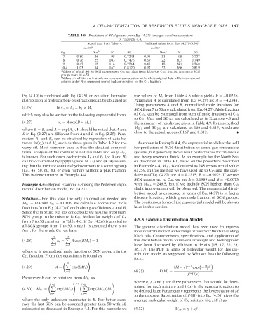
TABLE 4.9—Prediction of SCN groups from Eq. (4.27) for a gas condensate system
of Example 4.4.
Actual data from Table 4.1 Predicted values from Eqs. (4.27)–(4.30) a
mol% b mol% b
C N Nor. b M SG Nor. b M SG
7 0.80 26 95 0.7243 0.95 31 95 0.727
8 0.76 25 103 0.7476 0.69 22 107 0.749
9 0.47 15 116 0.7764 0.45 15 121 0.768
10+ 1.03 34 167 0.8120 0.97 32 166 0.819
a Values of M and SG for SCN groups up to C 50 are taken from Table 4.6. C 10+ fraction represents SCN
groups from 10 to 50.
b Values of mol% in the first column represent composition in the whole original fluid while in the second
column under Nor. represent normalized composition for the C 7+ fraction.
Eq. (4.10) is combined with Eq. (4.25), an equation for molar use values of M n from Table 4.6 which yields B =−0.0276.
distribution of hydrocarbon-plus fractions can be obtained as Parameter A is calculated from Eq. (4.29) as: A =−4.2943.
Using parameters A and B, normalized mole fractions for
(4.26) ln x n = A 1 + B 1 × M n SCN from 7 to 50 are calculated from Eq. (4.27). Mole fraction
which may also be written in the following exponential form. of C 10+ can be estimated from sum of mole fractions of C 10
to C 50 . M 10+ and SG 10+ are calculated as in Example 4.3 and
(4.27) x n = Aexp(B × M n ) the summary of results are given in Table 4.9. In this method
M 10+ and SG 10+ are calculated as 166 and 0.819, which are
where B = B 1 and A = exp(A 1 ). It should be noted that A and
B in Eq. (2.27) are different from A and B in Eq. (2.25). Para- close to the actual values of 167 and 0.812.
meters A 1 and B 1 can be obtained by regression of data be-
tween ln(x n ) and M n such as those given in Table 4.2 for the As shown in Example 4.4, the exponential model works well
waxy oil. Most common case is that the detailed composi- for prediction of SCN distribution of some gas condensate
systems, but generally shows weak performance for crude oils
tional analysis of the mixture is not available and only M 7+
is known. For such cases coefficients A 1 and B 1 (or A and B) and heavy reservoir fluids. As an example for the North Sea
can be determined by applying Eqs. (4.23) and (4.24) assum- oil described in Table 4.1, based on the procedure described
ing that the mixture contains hydrocarbons to a certain group in Example 4.4, M 10+ is calculated as 248 versus actual value
(i.e., 45, 50, 60, 80, or even higher) without a plus fraction. of 259. In this method we have used up to C 50 and the coef-
This is demonstrated in Example 4.4. ficients of Eq. (4.27) are A = 0.2215, B =−0.0079. If we use
SCN groups up to C 40 ,weget A = 0.1989 and B =−0.0073
Example 4.4—Repeat Example 4.3 using the Pedersen expo- with M 10+ = 246.5, but if we include SCN higher than C 50
nential distribution model, Eq. (4.27). slight improvement will be observed. The exponential distri-
bution model as expressed in terms of Eq. (4.27) is in fact a
Solution—For this case the only information needed are discrete function, which gives mole fraction of SCN groups.
M 7+ = 124 and x 7+ = 0.0306. We calculate normalized mole The continuous form of the exponential model will be shown
fractions from Eq. (4.27) after obtaining coefficients A and B. later in this section.
Since the mixture is a gas condensate we assume maximum
SCN group in the mixture is C 50 . Molecular weights of C N 4.5.3 Gamma Distribution Model
from 7 to 50 are given in Table 4.6. If Eq. (4.26) is applied to
all SCN groups from 7 to 50, since it is assumed there is no The gamma distribution model has been used to express
N 50+ , for the whole C 7+ we have molar distribution of wider range of reservoir fluids including
50 50 black oils. Characteristics, specifications, and application of

(4.28) x n = Aexp(BM n ) = 1 this distribution model to molecular weight and boiling point
n=7 n=7 have been discussed by Whitson in details [15, 17, 22, 23,
36, 37]. The PDF in terms of molecular weight for this dis-
where x n is normalized mole fraction of SCN group n in the
C 7+ fraction. From this equation A is found as tribution model as suggested by Whitson has the following
form:
−1

50

α−1 M−η
(4.29) A = exp(BM n ) (M − η) exp − β
n=7 (4.31) F(M) =
β (α)
α
Parameter B can be obtained from M 7+ as
where α, β, and η are three parameters that should be deter-
50 50

−1
mined for each mixture and (α) is the gamma function to
(4.30) M 7+ = exp(BM n ) [exp(BM n )]M n be defined later. Parameter η represents the lowest value of M
n=7 n=7
in the mixture. Substitution of F(M) into Eq. (4.20) gives the
where the only unknown parameter is B. For better accu- average molecular weight of the mixture (i.e., M 7+ ) as:
racy the last SCN can be assumed greater than 50 with M n
calculated as discussed in Example 4.2. For this example we (4.32) M 7+ = η + αβ

--`,```,`,``````,`,````,```,,-`-`,,`,,`,`,,`---
Copyright ASTM International
Provided by IHS Markit under license with ASTM Licensee=International Dealers Demo/2222333001, User=Anggiansah, Erick
No reproduction or networking permitted without license from IHS Not for Resale, 08/26/2021 21:56:35 MDT