Page 190 - Characterization and Properties of Petroleum Fractions - M.R. Riazi

QC: —/—
T1: IML
P2: KVU/KXT
P1: KVU/KXT
June 22, 2007
AT029-Manual
AT029-Manual-v7.cls
AT029-04
170 CHARACTERIZATION AND PROPERTIES OF PETROLEUM FRACTIONS
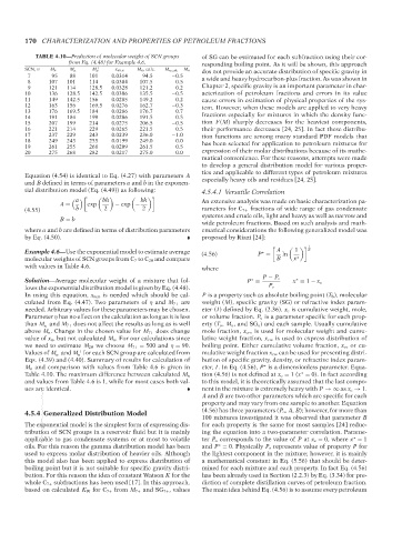
TABLE 4.10—Prediction of molecular weight of SCN groups
from Eq. (4.48) for Example 4.6. 21:30 of SG can be estimated for each subfraction using their cor-
responding boiling point. As it will be shown, this approach
SCN, n M n M n − M n + x av,n M n , calc. M n,calc − M n dos not provide an accurate distribution of specific gravity in
7 95 88 101 0.0314 94.5 −0.5 a wide and heavy hydrocarbon-plus fraction. As was shown in
8 107 101 114 0.0304 107.5 0.5
9 121 114 128.5 0.0328 121.2 0.2 Chapter 2, specific gravity is an important parameter in char-
10 136 128.5 142.5 0.0306 135.5 −0.5 acterization of petroleum fractions and errors in its value
11 149 142.5 156 0.0285 149.2 0.2 cause errors in estimation of physical properties of the sys-
12 163 156 169.5 0.0276 162.7 −0.3 tem. However, when these models are applied to very heavy
13 176 169.5 184 0.0286 176.7 0.7
14 191 184 199 0.0286 191.5 0.5 fractions especially for mixtures in which the density func-
15 207 199 214 0.0275 206.5 −0.5 tion F(M) sharply decreases for the heaviest components,
16 221 214 229 0.0265 221.5 0.5 their performance decreases [24, 25]. In fact these distribu-
17 237 229 243 0.0239 236.0 −1.0 tion functions are among many standard PDF models that
18 249 243 255 0.0199 249.0 0.0 has been selected for application to petroleum mixtures for
19 261 255 268 0.0209 261.5 0.5
20 275 268 282 0.0217 275.0 0.0 expression of their molar distributions because of its mathe-
matical convenience. For these reasons, attempts were made
to develop a general distribution model for various proper-
ties and applicable to different types of petroleum mixtures
Equation (4.54) is identical to Eq. (4.27) with parameters A
and B defined in terms of parameters a and b in the exponen- especially heavy oils and residues [24, 25].
tial distribution model (Eq. (4.49)) as following: 4.5.4.1 Versatile Correlation
a

bh bh An extensive analysis was made on basic characterization pa-
A = exp − exp −
(4.55) b 2 2 rameters for C 7+ fractions of wide range of gas condensate
systems and crude oils, light and heavy as well as narrow and
B = b
wide petroleum fractions. Based on such analysis and math-
where a and b are defined in terms of distribution parameters ematical considerations the following generalized model was
by Eq. (4.50). proposed by Riazi [24]:
1
B
Example 4.6—Use the exponential model to estimate average (4.56) P = A ln 1
∗
molecular weights of SCN groups from C 7 to C 20 and compare B x ∗
with values in Table 4.6. where
Solution—Average molecular weight of a mixture that fol- P = P − P ◦ x = 1 − x c
∗
∗
lows the exponential distribution model is given by Eq. (4.48). P ◦
In using this equation, x m,n is needed which should be cal- P is a property such as absolute boiling point (T b ), molecular
culated from Eq. (4.47). Two parameters of η and M 7+ are weight (M), specific gravity (SG) or refractive index param-
needed. Arbitrary values for these parameters may be chosen. eter (I) defined by Eq. (2.36). x c is cumulative weight, mole,
Parameter η has no effect on the calculation as long as it is less or volume fraction. P o is a parameter specific for each prop-
than M and M 7+ does not affect the results as long as is well erty (T o , M o , and SG o ) and each sample. Usually cumulative
−
n
above M n . Change in the chosen value for M 7+ does change mole fraction, x cm is used for molecular weight and cumu-
value of x n , but not calculated M n . For our calculations since lative weight fraction, x cw is used to express distribution of
we need to estimate M 20 we choose M 7+ = 500 and η = 90. boiling point. Either cumulative volume fraction, x cv or cu-
Values of M and M for each SCN group are calculated from mulative weight fraction x cw can be used for presenting distri-
−
+
n n
Eqs. (4.39) and (4.40). Summary of results for calculation of bution of specific gravity, density, or refractive index param-
M n and comparison with values from Table 4.6 is given in eter, I. In Eq. (4.56), P is a dimensionless parameter. Equa-
∗
tion (4.56) is not defined at x c = 1(x = 0). In fact according
∗
Table 4.10. The maximum difference between calculated M n
and values from Table 4.6 is 1, while for most cases both val- to this model, it is theoretically assumed that the last compo-
ues are identical. nent in the mixture is extremely heavy with P →∞ as x c → 1.
A and B are two other parameters which are specific for each
property and may vary from one sample to another. Equation
(4.56) has three parameters (P o , A, B); however, for more than
4.5.4 Generalized Distribution Model
100 mixtures investigated it was observed that parameter B
The exponential model is the simplest form of expressing dis- for each property is the same for most samples [24] reduc-
tribution of SCN groups in a reservoir fluid but it is mainly ing the equation into a two-parameter correlation. Parame-
applicable to gas condensate systems or at most to volatile ter P o corresponds to the value of P at x c = 0, where x = 1
∗
--`,```,`,``````,`,````,```,,-`-`,,`,,`,`,,`---
oils. For this reason the gamma distribution model has been and P = 0. Physically P o represents value of property P for
∗
used to express molar distribution of heavier oils. Although the lightest component in the mixture; however, it is mainly
this model also has been applied to express distribution of a mathematical constant in Eq. (5.56) that should be deter-
boiling point but it is not suitable for specific gravity distri- mined for each mixture and each property. In fact Eq. (4.56)
bution. For this reason the idea of constant Watson K for the has been already used in Section (2.2.3) by Eq. (3.34) for pre-
whole C 7+ subfractions has been used [17]. In this approach, diction of complete distillation curves of petroleum fraction.
based on calculated K W for C 7+ from M 7+ and SG 7+ , values The main idea behind Eq. (4.56) is to assume every petroleum

Copyright ASTM International
Provided by IHS Markit under license with ASTM Licensee=International Dealers Demo/2222333001, User=Anggiansah, Erick
No reproduction or networking permitted without license from IHS Not for Resale, 08/26/2021 21:56:35 MDT