Page 195 - Characterization and Properties of Petroleum Fractions - M.R. Riazi

P2: KVU/KXT
T1: IML
QC: —/—
P1: KVU/KXT
21:30
June 22, 2007
AT029-04
AT029-Manual-v7.cls
AT029-Manual
4. CHARACTERIZATION OF RESERVOIR FLUIDS AND CRUDE OILS 175
It is much easier to work in terms of P rather than P, since for
∗
any mixture P starts at 0. However, based on the definition Carbon Number, N C
∗
of P in Eq. (4.56), the PDF expressed by Eq. (4.66) can be 5 10 15 20 25
∗
written in terms of original property P. Since dx = F(P)dP = 0.018
F(P )dP and dP = P o dP , therefore we have
∗
∗
∗
Generalized Model
B=2
1 Gamma Model
(4.69) F(P) = F(P )
∗
P ◦ 0.012
Substituting F(P ) from Eq. (4.66) into the above equation
∗
and use of definition of P we get Density Function, F(M) B=1 B=3
∗
1 B P − P ◦ B P − P ◦
2 B−1 B
F(P) = × × exp − 0.006
A A
P ◦ P ◦ P ◦ B=0.7
(4.70)
with this form of PDF, Eq. (4.18) should be used to calcu-
late cumulative, x c at P. Obviously it is more convenient to 0
work in terms of P through Eq. (4.68) and at the end P can 80 160 240 320
∗
∗
be converted to P. This approach is used for calculation of
average properties in the next section. Molecular Weight, M
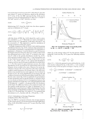
A simple comparison of Eq. (4.70) or (4.66) with the gamma FIG. 4.16—Comparison of Eqs. (4.31) and Eq. (4.66)
distribution function, Eq. (4.31), indicates that parameter P o for M o = η = 90, B = αα, and M 7+ = 150.
is equivalent to parameter η and parameter B is equivalent to
parameter α. Parameter A can be related to α and β; however,
the biggest difference between these two models is that inside where P is the average value of P for the mixture. Substi-
∗
∗
av
the exponential term in Eq. (4.66), P is raised to the expo- tuting Eq. (4.66) into Eq. (4.71) gives the following relation
∗
nent B, while in the gamma distribution model, Eq. (4.31), for P :
∗
av
such exponent is always unity. At B = 1, the exponential term 1
in Eq. (4.66) becomes similar to that of Eq. (4.31). In fact (4.72) ∗ A B 1
av
at B = 1, Eq. (4.66) reduces to the exponential distribution P = B 1 + B
model as was the case for the gamma distribution model when
α = 1. For this reason for gas condensate systems, the molar where (1 + 1/B) is the gamma function defined by Eq. (4.43)
distribution can be presented by an exponential model as the and may be evaluated by Eq. (4.44) with x = 1/B. A simpler
behavior of two models is the same. However, for molar dis- version of Eq. (4.44) was given in Chapter 3 by Eq. (3.37) as
tribution of heavy oils or for properties other than molecular 1 −1 −2
weight in which parameter B is greater than 1, the difference 1 + B = 0.992814 − 0.504242B + 0.696215B
between two models become more apparent. As it is shown in (4.73) − 0.272936B −3 + 0.088362B −4
Section 4.5.4.5, the molar distribution of very heavy oils and
residues is best presented by the generalized model (Eq. 4.66).
For the same reason Eq. (4.66) is applicable for presentation Carbon Number, N
of other properties such as specific gravity or refractive index 5 10 15 C 20 25
as it is shown in Section 4.5.4.4. A comparison between the
gamma distribution model (Eq. 4.31) and generalized model 0.018
(4.70) when M o = η and B = α is shown in Fig. 4.16. As shown
in this figure the difference between the proposed model and 2 2.5
the gamma model increases as value of parameter B or α 3
(keeping them equal) increases. Effect of parameter B on the 0.012
form and shape of distribution model by Eq. (4.70) is shown 1.5
in Fig. 4.17. For both Figs. 4.16 and 4.17, it is assumed that Density Function, F(M)
the mixture is a C 7+ fraction with M o = 90 and M 7+ = 150. 1
4.5.4.3 Calculation of Average Properties 0.006
of Hydrocarbon-Plus Fractions 0.7
Once the PDF for a property is known, the average property
for the whole mixture can be determined through application 5
of Eq. (4.20). If the PDF in terms of P is used, then Eq. (4.20) 0
∗
becomes 80 160 240 320
Molecular Weight, M
∞

(4.71) P = P F(P )dP ∗ FIG. 4.17—Effect of parameter B on the shape of
∗
∗
∗
av
--`,```,`,``````,`,````,```,,-`-`,,`,,`,`,,`---
0 Eq. (4.70) for M o = 90 and M 7+ = 150.
Copyright ASTM International
Provided by IHS Markit under license with ASTM Licensee=International Dealers Demo/2222333001, User=Anggiansah, Erick
No reproduction or networking permitted without license from IHS Not for Resale, 08/26/2021 21:56:35 MDT