Page 194 - Characterization and Properties of Petroleum Fractions - M.R. Riazi

QC: —/—
P2: KVU/KXT
T1: IML
P1: KVU/KXT
21:30
June 22, 2007
AT029-Manual-v7.cls
AT029-Manual
AT029-04
174 CHARACTERIZATION AND PROPERTIES OF PETROLEUM FRACTIONS
10
4
8
3
PDF, F(T b*) 2 PDF, F(SG * ) 6
1 4
2
0
0 0.2 0.4 0.6 0.8 1 0
T * 0 0.1 0.2 0.3 0.4
b
SG *
0.012
14
12
0.009 10
PDF, F(T b ) 0.006 PDF, F(SG) 8

0.003 6
4
2
0
300 400 500 600 700 800 0
0.7 0.8 0.9 1
Boiling Point, T , K Specific Gravity, SG
b
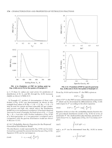
FIG. 4.14—Prediction of PDF for boiling point by FIG. 4.15—Prediction of PDF for specific gravity by
Eqs. (4.66) and (4.70) for the system of Example 4.7.
Eqs. (4.66) and (4.70) for the system of Example 4.7.
to 3. If these fix values are used errors for prediction of From Eq. (4.16) and in terms P , the PDF is given as
∗
distribution of M, T b , and SG through Eq. (4.56) increases
slightly as shown in Table 4.13. (4.65) F(P ) = dx c
∗
dP ∗
∗
In Example 4.7, method of determination of three coef- where F(P ) is the PDF in terms of dimensionless parameter
∗
ficients of Eq. (4.56) was demonstrated. As shown in this P which can be determined by differentiation of Eq. (4.64)
∗
example fixed values of B (B M = 1, B T = 1.5, B SG = 3, B I = 3) with respect to P according to the above equation:
may be used for certain mixtures especially for gas conden- B 2 ∗B−1 B ∗B
∗
sate systems and light oils, which reduce the distribution (4.66) F(P ) = A P exp − A P
model into a two-parameter correlation. It has been observed
--`,```,`,``````,`,````,```,,-`-`,,`,,`,`,,`---
that even for most oil samples the fixed values of B T = 1.5 and Equation (4.66) is in fact the probability density function for
B SG = B I = 3 are also valid. Further evaluation of Eq. (4.56) the generalized distribution model of Eq. (4.56) in terms of
∗
as a three-parameter or a two-parameter correlation and a parameter P . In a hydrocarbon plus fraction, parameter P ∗
comparison with the gamma distribution model are shown varies from 0 to ∞. Application of Eq. (4.17) in terms of P ∗
in Section 4.5.4.5. gives:
∞

4.5.4.2 Probability Density Function for the Proposed (4.67) F(P )dP = 1
∗
∗
Generalized Distribution Model
0
The distribution model expressed by Eq. (4.56) can be trans- and x c at P can be determined from Eq. (4.18) in terms
∗
formed into a probability density function by use of Eq. (4.16). of P :
∗
Equation (4.56) can be rearranged as
∗
P
B (4.68) x c = F(P )dP ∗
∗

(4.64) 1 − x c = exp − P ∗B
A 0

Copyright ASTM International
Provided by IHS Markit under license with ASTM Licensee=International Dealers Demo/2222333001, User=Anggiansah, Erick
No reproduction or networking permitted without license from IHS Not for Resale, 08/26/2021 21:56:35 MDT