Page 192 - Characterization and Properties of Petroleum Fractions - M.R. Riazi

P2: KVU/KXT
QC: —/—
T1: IML
P1: KVU/KXT
AT029-04
AT029-Manual-v7.cls
June 22, 2007
21:30
AT029-Manual
172 CHARACTERIZATION AND PROPERTIES OF PETROLEUM FRACTIONS
40
M 1 (molecular weight of the first component in the mixture).
The best value for M o is the lower molecular weight boundary
for C 7 group that is M in Table 4.10, which is 88. Similarly
−
7
Discrete Mole Percent 20 0.7 for the initial guesses of M o , T bo , and SG o , respectively.
the best initial guess for T bo and SG o are 351 K and 0.709,
30
respectively. These numbers can be simplified to 90, 350, and
Similarly for a C 6+ fraction, the initial guess for its M o can be
taken as the lower molecular weight boundary for C 6 (M ).
−
6
For this example, based on the value of M o = 90, parameters
Y i and X i are calculated and are given in Table 4.12. A linear
regression gives values of C 1 and C 2 and from Eq. (4.58) pa-
10
rameters A and B are calculated which are given in Table 4.12.
For these values of M o , A, and B, values of M i are calculated
from Eq. (4.56) and the error function E(M o ) and AAD% are
0
0 25 50 75 100 calculated as 2.7 and 1.32, respectively. Value of M o should
be changed so that E(M o ) calculated from Eq. (4.59) is mini- --`,```,`,``````,`,````,```,,-`-`,,`,,`,`,,`---
Cumulative Mole Percent mized. As shown in Table 4.12, the best value for this sam-
ple is M o = 91 with A = 0.2854 and B = 0.9429. These co-
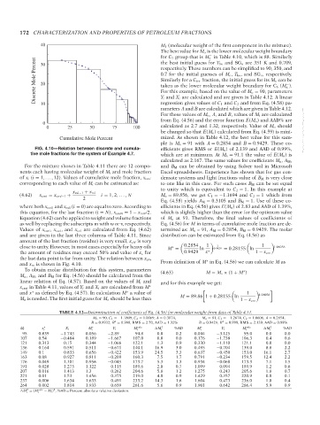
FIG. 4.10—Relation between discrete and cumula- efficients gives RMS or E(M o ) of 2.139 and AAD of 0.99%,
tive mole fractions for the system of Example 4.7. which are at minimum. At M o = 91.1 the value of E(M o )is
calculated as 2.167. The same values for coefficients M o , A M ,
For the mixture shown in Table 4.11 there are 12 compo- and B M can be obtained by using Solver tool in Microsoft
nents each having molecular weight of M i and mole fraction Excel spreadsheets. Experience has shown that for gas con-
of x i (i = 1,..., 12). Values of cumulative mole fraction, x cmi densate systems and light fractions value of B M is very close
corresponding to each value of M i can be estimated as: to one like in this case. For such cases B M can be set equal
to unity which is equivalent to C 2 = 1. In this example at
x mi−1 + x mi
(4.62) x cmi = x cmi−1 + i = 1, 2, ... , N M o = 89.856, we get C 1 =−1.1694 and C 2 = 1 which from
2
Eq. (4.58) yields A M = 0.3105 and B M = 1. Use of these co-
where both x cm0 and x m0 (i = 0) are equal to zero. According to efficients in Eq. (4.56) gives E(M o ) of 2.83 and AAD of 1.39%,
this equation, for the last fraction (i = N), x cmN = 1 − x mN /2. which is slightly higher than the error for the optimum value
Equation (4.62) can be applied to weight and volume fractions of M o at 91. Therefore, the final values of coefficients of
as well by replacing the subscripts m with w or v, respectively. Eq. (4.56) for M in terms of cumulative mole fraction are de-
Values of x cmi , x cwi , and x cvi are calculated from Eq. (4.62) termined as: M o = 91, A M = 0.2854, B M = 0.9429. The molar
and are given in the last three columns of Table 4.11. Since distribution can be estimated from Eq. (4.56) as
amount of the last fraction (residue) is very small, x cN is very

1
close to unity. However, in most cases especially for heavy oils M = 0.2854 ln 1 0.9429 = 0.28155 ln 1 1.06056
∗
the amount of residues may exceed 50% and value of x c for 0.9429 x ∗ 1 − x cm
the last data point is far from unity. The relation between x cm ∗
and x m is shown in Fig. 4.10. From definition of M in Eq. (4.56) we can calculate M as
To obtain molar distribution for this system, parameters (4.63) M = M ◦ × (1 + M )
∗
M o , A M , and B M for Eq. (4.56) should be calculated from the
linear relation of Eq. (4.57). Based on the values of M i and and for this example we get:
x cmi in Table 4.11, values of Y i and X i are calculated from M ∗
and x as defined by Eq. (4.57). In calculation M a value of 1 1.06056
∗
∗
M o is needed. The first initial guess for M o should be less than M = 89.86 1 + 0.28155 ln
1 − x cm
TABLE 4.12—Determination of coefficients of Eq. (4.56) for molecular weight from data of Table 4.11.
M o = 90, C 1 =−1.1809, C 2 = 1.0069, A = 0.3074, M o = 91, C 1 =−1.2674, C 2 = 1.0606, A = 0.2854,
2
2
B = 0.9932, R = 0.998, RMS = 2.70, AAD = 1.32% B = 0.9429, R = 0.999, RMS = 2.139, AAD = 0.99%
M i x ∗ i X i M i ∗ Y i M calc M 2 i %AD M ∗ i Y i M i calc M i 2 %AD
i
95 0.839 −1.743 0.056 −2.89 94.8 0.0 0.2 0.044 −3.125 95.0 0.0 0.0
107 0.54 −0.484 0.189 −1.667 107.0 0.0 0.0 0.176 −1.738 106.3 0.4 0.6
121 0.313 0.15 0.344 −1.066 122.1 1.3 0.9 0.330 −1.110 121.1 0.0 0.0
136 0.164 0.591 0.511 −0.671 140.1 16.9 3.0 0.495 −0.704 139.0 8.8 2.2
149 0.1 0.833 0.656 −0.422 153.9 24.5 3.3 0.637 −0.450 153.0 16.1 2.7
163 0.08 0.927 0.811 −0.209 160.3 7.5 1.7 0.791 −0.234 159.5 12.4 2.2
176 0.049 1.101 0.956 −0.045 173.7 5.3 1.3 0.934 −0.068 173.3 7.1 1.5
191 0.028 1.273 1.122 0.115 189.6 2.0 0.7 1.099 0.094 189.9 1.2 0.6
207 0.016 1.413 1.3 0.262 204.6 5.8 1.2 1.275 0.243 205.6 1.8 0.7
221 0.01 1.53 1.456 0.375 219.0 4.0 0.9 1.429 0.357 220.9 0.0 0.1
237 0.006 1.634 1.633 0.491 233.2 14.3 1.6 1.604 0.473 236.0 1.0 0.4
264 0.002 1.814 1.933 0.659 261.6 5.6 0.9 1.901 0.642 266.4 5.9 0.9
2
2
M = (M calc − M i ) ,%AD = Percent absolute relative deviation.
i
i
Copyright ASTM International
Provided by IHS Markit under license with ASTM Licensee=International Dealers Demo/2222333001, User=Anggiansah, Erick
No reproduction or networking permitted without license from IHS Not for Resale, 08/26/2021 21:56:35 MDT