Page 188 - Characterization and Properties of Petroleum Fractions - M.R. Riazi

P1: KVU/KXT
AT029-Manual-v7.cls
June 22, 2007
AT029-04
AT029-Manual
168 CHARACTERIZATION AND PROPERTIES OF PETROLEUM FRACTIONS
which can be used to estimate parameter β in the following
form. P2: KVU/KXT QC: —/— T1: IML 21:30 250
M 7+ − η
(4.33) β =
α 200
Whitson et al. [37] suggest an approximate relation between
η and α as follows:
1 150

(4.34) η = 110 1 − Molecular Weight, M
1 + 4.043α −0.723
By substituting Eq. (4.31) into Eq. (4.18), cumulative mole
fraction, x cm versus molecular weight, M can be obtained 100
which in terms of an infinite series is given as:

∞ M α+1
b
(4.35) x cm = [exp(−M b )] 50
j=0 (α + 1 + j) 7 9 11 13 15
where parameter M b is a variable defined in terms of M as
Carbon Number, C N
M − η
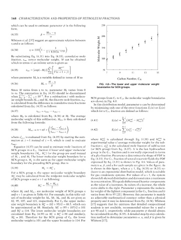
(4.36) M b = FIG. 4.8—The lower and upper molecular weight
β
boundaries for SCN groups.
Since M varies from η to ∞, parameter M b varies from 0
to ∞. The summation in Eq. (4.35) should be discontinued
when J+1 − J j=0 ≤ 10 . For a subfraction i with molecu- SCN groups from C 7 to C 15 the molecular weight boundaries
−8
j=0
lar weight bounds M i−1 and M i , the discrete mole fraction, x m,i are shown in Fig. 4.8.
is calculated from the difference in cumulative mole fractions In this distribution model, parameter α can be determined
calculated from Eq. (4.35) as follows:
by minimizing only one of the error functions E 1 (α)or E 2 (α)
(4.37) x m,i = x cm,i − x cm,i−1 which for a C 7+ fraction are defined as follows:
where M bi is calculated from Eq. (4.36) at M i . The average N−1
molecular weight of this subfraction, M av,i is then calculated (4.41) E 1 (α) = M cal − M exp 2

from the following formula: i=7 av,i av,i
x cm,i − x cm,i−1 exp 2

1 1 N−1
(4.38) M av,i = η + αβ × (4.42) E 2 (α) = x cal − x m,i
m,i
x cm,i − x cm,i−1
i=7
where x cm,i is evaluated from Eq. (4.35) by starting the sum- cal exp
1
mation at j = 1 instead of j = 0, which is used to evaluate where M av,i is calculated through Eq. (4.38) and M av,i is
x cm,i . experimental value of average molecular weight for the sub-
cal
Equation (4.37) can be used to estimate mole fractions of fraction i. x m,i is the calculated mole fraction of subfraction
SCN groups in a C 7+ fraction if lower and upper molecular (or SCN group) from Eq. (4.37). N is the last hydrocarbon
weight boundaries (M , M ) for the group are used instead group in the C 7+ fraction and is normally expressed in terms
+
−
n
n
of M i−1 and M i. The lower molecular weight boundary for a of a plus fraction. Parameter α determines the shape of PDF in
SCN group n, M is the same as the upper molecular weight Eq. (4.31). For C 7+ fraction of several reservoir fluids the PDF
−
n
boundary for the preceding SCN group, that is expressed by Eq. (4.31) is shown in Fig. 4.9. Values of para-
meters α, β, and η for each sample are given in the figure. As
(4.39) M = M + is shown in this figure, when α ≤ 1, Eq. (4.35) or (4.31) re-
−
n
n−1
For a SCN group n, the upper molecular weight boundary duces to an exponential distribution model, which is suitable
M may be calculated from the midpoint molecular weights for gas condensate systems. For values of α> 1, the system
+
n
of SCN groups n and n + 1 as following: shows left-skewed distribution and demonstrates a maximum
in concentration. This peak shifts toward heavier components
M n + M n+1 as the value of α increases. As values of η increase, the whole
(4.40) M =
+
n 2 curve shifts to the right. Parameter η represents the molecu-
where M n and M n+1 are molecular weight of SCN groups n lar weight of the lightest component in the C 7+ fraction and it
and n + 1 as given in Table 4.6. For example, in this table val- varies from 86 to 95 [23]. However, this parameter is mainly
ues of molecular weight for M 6 , M 7 , M 8 , and M 9 are given as an adjustable mathematical constant rather than a physical
--`,```,`,``````,`,````,```,,-`-`,,`,,`,`,,`---
82, 95, 107, and 121, respectively. For C 6 the upper molec- property and it may be determined from Eq. (4.34). Whitson
ular weight boundary is M = (82 + 95)/2 = 88.5, which can [17] suggests that for mixtures that detailed compositional
+
6
be approximated as 88. Similarly, M = (95 + 107)/2 = 101 analysis is not available, recommended values for η and α
+
7
and M = 114. The lower molecular weight boundaries are are 90 and 1, respectively, while parameter β should always
+
8
calculated from Eq. (4.39) as M = M = 88 and similarly, be calculated from Eq. (4.33). A detailed step-by-step calcula-
+
−
6
7
M = 101. Therefore for the SCN group of C 8 , the lower tion method to determine parameters α, η, and β is given by
−
8
molecular weight is 101 and the upper boundary is 114. For Whitson [17].
Copyright ASTM International
Provided by IHS Markit under license with ASTM Licensee=International Dealers Demo/2222333001, User=Anggiansah, Erick
No reproduction or networking permitted without license from IHS Not for Resale, 08/26/2021 21:56:35 MDT