Page 290 - Characterization and Properties of Petroleum Fractions - M.R. Riazi

P2: KVU/KXT
T1: IML
P1: KVU/KXT
QC: —/—
June 22, 2007
AT029-Manual-v7.cls
AT029-06
AT029-Manual
270 CHARACTERIZATION AND PROPERTIES OF PETROLEUM FRACTIONS

(a) 20:46 (b)
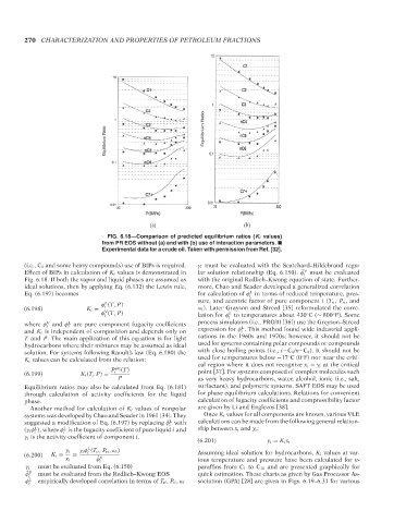
FIG. 6.18—Comparison of predicted equilibrium ratios (K i values)
from PR EOS without (a) and with (b) use of interaction parameters.
Experimental data for a crude oil. Taken with permission from Ref. [32].

(i.e., C 1 and some heavy compounds) use of BIPs is required. γ i must be evaluated with the Scatchard–Hildebrand regu-
V
Effect of BIPs in calculation of K i values is demonstrated in lar solution relationship (Eq. 6.150). ˆ φ must be evaluated
i
Fig. 6.18. If both the vapor and liquid phases are assumed as with the original Redlich–Kwong equation of state. Further-
ideal solutions, then by applying Eq. (6.132) the Lewis rule, more, Chao and Seader developed a generalized correlation
L
Eq. (6.197) becomes for calculation of φ in terms of reduced temperature, pres-
i
sure, and acentric factor of pure component i (T ri , P ri , and
L
φ (T, P)
(6.198) K i = i ω i ). Later Grayson and Streed [35] reformulated the corre-
V
φ (T, P) lation for φ to temperatures about 430 C(∼ 800 F). Some
L
◦
◦
i
i
V
where φ and φ are pure component fugacity coefficients process simulators (i.e., PRO/II [36]) use the Greyson–Streed
L
i
i
L
and K i is independent of composition and depends only on expression for φ . This method found wide industrial appli-
i
T and P. The main application of this equation is for light cations in the 1960s and 1970s; however, it should not be
hydrocarbons where their mixtures may be assumed as ideal used for systems containing polar compounds or compounds
solution. For systems following Raoult’s law (Eq. 6.180) the with close boiling points (i.e., i−C 4 /n−C 4 ). It should not be
◦
◦
K i values can be calculated from the relation: used for temperatures below −17 C(0 F) nor near the criti-
cal region where it does not recognize x i = y i at the critical
P sat (T)
(6.199) K i (T, P) = i point [37]. For systems composed of complex molecules such
P as very heavy hydrocarbons, water, alcohol, ionic (i.e., salt,
Equilibrium ratios may also be calculated from Eq. (6.181) surfactant), and polymeric systems, SAFT EOS may be used
through calculation of activity coefficients for the liquid for phase equilibrium calculations. Relations for convenient
phase. calculation of fugacity coefficients and compressibility factor
Another method for calculation of K i values of nonpolar are given by Li and Englezos [38].
systems was developed by Chao and Seader in 1961 [34]. They Once K i values for all components are known, various VLE
L
suggested a modification of Eq. (6.197) by replacing ˆ φ with calculations can be made from the following general relation-
i
L
L
(γ i φ ), where φ is the fugacity coefficient of pure liquid i and ship between x i and y i :
i
i
γ i is the activity coefficient of component i.
(6.201) y i = K i x i
L
y i γ i φ (T ri , P ri , ω i ) Assuming ideal solution for hydrocarbons, K i values at var-
i
(6.200) K i = = V
x i ˆ φ ious temperature and pressure have been calculated for n-
i
γ i must be evaluated from Eq. (6.150) paraffins from C 1 to C 10 and are presented graphically for
ˆ φ V must be evaluated from the Redlich–Kwong EOS quick estimation. These charts as given by Gas Processor As-
i
φ L sociation (GPA) [28] are given in Figs. 6.19–6.31 for various
i empirically developed correlation in terms of T ri , P ri , ω i
--`,```,`,``````,`,````,```,,-`-`,,`,,`,`,,`---
Copyright ASTM International
Provided by IHS Markit under license with ASTM Licensee=International Dealers Demo/2222333001, User=Anggiansah, Erick
No reproduction or networking permitted without license from IHS Not for Resale, 08/26/2021 21:56:35 MDT