Page 398 - Characterization and Properties of Petroleum Fractions - M.R. Riazi

QC: IML/FFX
P2: IML/FFX
T1: IML
P1: IML/FFX
AT029-Manual-v7.cls
AT029-Manual
AT029-09
June 22, 2007
14:25
378 CHARACTERIZATION AND PROPERTIES OF PETROLEUM FRACTIONS
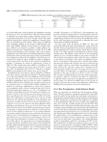
TABLE 9.8—Evaluation of three types of additives for asphaltene removal on a rock surface [37].
Removal efficiency (wt% of adsorbed asphaltene)
for different additives
Additive wt% in solvent Time, h Additive A Additive B Additive C
0.1 1 40.5 14.0 2.7
0.1 18 48.9 21.4 6.0
2.0 1 49.9 32.9 8.9
2.0 18 51.5 46.0 10.1
are in the bulk state; on the contrary, the asphaltene up-take example, Kawanaka et al. [30] used a thermodynamic ap-
by toluene is very low (10–20 wt%) when the same material proach to study the phase behavior and deposition region in
is adsorbed on a rock surface (clays, dolomia, quartz, etc.), CO 2 –crude mixtures at different pressures, temperatures, and
as experienced by Piro et al. [37]. For this reason, they used compositions. In the next few sections, thermodynamic mod-
additives dissolved in toluene for asphaltenes’ removal when els for solid formation are presented to calculate the onset
they are adsorbed on rock surface. Three types of additives and amount of solid precipitation.
were evaluated: additive A was based on alkyl benzene sul- For the same tank oil shown in Table 9.9, Pan and
fonic acid (ABSA); additive B was based on complex poly- Firoozabai [20] used their thermodynamic model based on
mer; additive C was based on another complex polymer. As- micellar theory of asphaltene formation to calculate asphal-
phaltic materials were obtained from a crude oil of 42 API tene precipitation for various solvents. Their data are shown
gravity by precipitation with n-heptane. The rock on which in Fig. 9.12, where amount of precipitation is shown versus
asphaltenes were adsorbed was powdered dolomite (average dilution ratio. The dilution ratio (shown by R S ) represents
3
2
particle size of 60 μm and surface area of 10 m /g) and toluene volume (in cm ) of solvent added to each gram of crude oil.
was employed as solvent for the additives. Experiments were The amount of precipitated resin under the same conditions
conducted to study the effect of different types of additives, is also shown in this figure. The onset of asphaltene forma-
concentration level, and time on the amount of asphaltenes tion is clearly shown at the point where amount of precipita-
up-take. A summary of results of experiments is given in tion does not change with a further increase in solvent-to-oil
Table 9.8. The results show that addition of additive A (0.1 ratio. Lighter solvents cause higher precipitation. Generally
wt% in toluene solution) can remove up to 41% after 1 h and value of R S at the onset for a given oil is a function of sol-
up to 49% of asphaltene after 18 h [37]. Therefore, at higher vent molecular weight (M S ) and it increases with increase in
additive concentrations the contact time can be reduced. M S [38]. Effect of temperature on asphaltene precipitation
Deasphalted oils may also be used as asphaltene inhibitor depends on the type of solvent as shown in Fig. 9.13 [39].
since they contain resins that are effective in keeping asphal- The amount of solid deposition increases with temperature
tene molecules soluble in the oil in addition to their potential for propane, while for n-heptane the effect of temperature
for greater solvency. There are some synthetic resins such 2- is opposite. Effect of pressure on asphaltene precipitation is
hexadecyl naphthalene that can also be used as asphaltene shown in Fig. 9.14. Above the bubble point of oil, increase in
inhibitor. Most of these inhibitors are expensive and research pressure decreases the amount of precipitation, while below
on manufacturing of commercially feasible asphaltene in- bubble point precipitation increases with pressure.
hibitors is continuing. Asphaltenes or other heavy organics
are precipitated under certain conditions that can be deter- 9.3.2 Wax Precipitation—Solid Solution Model
mined through phase diagram (i.e., PT or Px diagrams). An
example of such diagrams is the Px diagram at constant tem- There are generally two models for wax formation calcula-
perature of 24 C for an oil–CO 2 system as shown in Fig. 9.11. tions. The first and more commonly used model is the solid-
◦
Some specifications for this oil are given in Table 9.9. In this solution model. In this model, the solid phase is treated as a
figure, the solid phase is indicated by S and regions of LVS homogenous solution similar to liquid solutions. Formulation
and LS are the regions that asphaltenes may precipitate and of SLE calculations according to this model is very similar
should be avoided. The best way to prevent asphaltene pre- to VLE calculations with use of Eq. (6.205) and equilibrium --`,```,`,``````,`,````,```,,-`-`,,`,,`,`,,`---
cipitation is to avoid the region in the phase diagram where ratio, K , from Eq. (6.209) instead of K i for the VLE. This
SL
i
asphaltene precipitation can occur. It is for this reason that model was first introduced by Won [41] and later was used
phase behavior of petroleum fluids containing heavy organics to predict wax precipitation from North Sea oils by Pedersen
is important in determining the conditions in which precipi- et al. [14, 42]. The second model called multisolid-phase model
tation can be avoided. Construction of such phase diagrams was proposed by Lira-Galeana et al. in 1996 [43], which has
is extremely useful to determine the conditions where precip- also found some industrial applications [16]. In this model,
itation occurs. Unfortunately such diagrams for various oils the solid mixture is not considered as a solution but it is de-
and solvents are not cited in the open literature. Figure 9.11 scribed as a mixture of pure components; each solid phase
shows that the solid phase is formed at very high concentra- does not mix with other solid phases. The multisolid-phase
tion of CO 2 , that is, the region that is not of practical applica- model is particularly useful for calculation of CPT of oils.
tion and should be considered with caution. Thermodynamic The temperature at which wax appears is known as wax ap-
models, along with appropriate characterization schemes can pearance (or precipitation) temperature (WAT or WPT), which
be applied to waxy or asphaltic oils to determine possibility theoretically is the same as the CPT. Both models are based on
and amount of precipitation under certain conditions. For the following relation expressing equilibrium between vapor,

Copyright ASTM International
Provided by IHS Markit under license with ASTM Licensee=International Dealers Demo/2222333001, User=Anggiansah, Erick
No reproduction or networking permitted without license from IHS Not for Resale, 08/26/2021 21:56:35 MDT