Page 400 - Characterization and Properties of Petroleum Fractions - M.R. Riazi

P2: IML/FFX
QC: IML/FFX
P1: IML/FFX
AT029-Manual
AT029-09
AT029-Manual-v7.cls
June 22, 2007
380 CHARACTERIZATION AND PROPERTIES OF PETROLEUM FRACTIONS
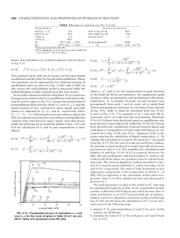
TABLE 9.9—Data for shell tank oil of Fig. 9.12 [30].
Oil specifications T1: IML 14:25 Asphaltene specifications
mol% C 1 + C 2 0.6 wt% (resin) in oil 14.1 a
mol% C 3 –C 5 10.6 wt% (asph.) in oil 4.02
mol% C 6 4.3 density, g/cm 3 1.2
84.5
mol% C 7+
M 221.5 (M 7+ = 250) M (precipitated) b 4500
SG 0.873 (SG 7+ = 0.96) a δ c T 12.66(1 – 8.28 × 10 −4 T)
a Data taken from Refs. [20, 49].
b M for asphaltene in oil (monomer) is about 1000 [20].
3 0.5
c δ in (cal/cm ) and T in kelvin.
N z i K VL
liquid, and solid phases for a multicomponent system shown (9.18) y i = i

in Fig. 9.15. i=1 (1 − S F ) + V F K i VL − 1
N N z i K SL − 1

ˆ V

(9.15) f (T, P, y i ) = f ˆ L T, P, x L = f ˆ S T, P, x S SL S L i
i i i i i (9.19) F = x − x i = SL = 0
i
i=1 i=1 1 + S F K i − 1
This equation can be split into two parts, one for vapor–liquid
L
equilibrium and the other for liquid–solid equilibrium. These (9.20) x = z i SL
i
two equations can be expressed by two relations in terms of 1 + S F K i − 1
equilibrium ratios as given by Eqs. (6.201) and (6.208). In (9.21) x = x K SL
S
L
this section the solid-solution model is discussed while the i i i
S
L
multisolid-phase model is presented in the next section. where z i , x , and x are the compositions in mole fractions
i
i
In the solid-solution model the solid phase (S) is treated as a of the crude oil (before precipitation), the equilibrium liquid
homogeneous solution that is in equilibrium with liquid solu- oil phase (after precipitation), and precipitated solid phase,
tion (L) and its vapor. In Fig. 9.15, assume the initial moles of respectively. S F is number of moles of solid formed (wax
nonequilibrium fluid mixture (feed) is 1 mol (F = 1) and the precipitated) from each 1 mol of crude oil or initial fluid
molar fraction of feed converted to vapor, liquid, and solid (before precipitation) and must be calculated from solution
phases are indicated by V F , L F , and S F , respectively, where of Eq. (9.9), while V F must be calculated from Eq. (9.16).
L F = 1 − V F − S F . Following the same procedure as that in the In fact in Fig. 9.15, F is assumed to be 1 mol and 100 S F
VLE calculations and using the mass balance and equilibrium represents mol% of crude that has precipitated. Equations
relations that exist between vapor, liquid, and solid phases (9.16)–(9.18) have been developed based on equilibrium rela-
yields the following set of equations similar to Eqs. (9.3) and tions between vapor and liquid, while Eqs. (9.19)–(9.21) have
(9.4) for calculation of V F and S F and compositions of three been derived from equilibrium relations between liquid and
phases: solid phases. Compositions of vapor and solid phases are cal-
culated from Eqs. (9.18) and (9.21). Equation (9.20) is the
N N z i K VL − 1 prime equation for calculation of liquid composition, x .To
L

i
(9.16) F VL = y i − x i L = i VL = 0 validate the calculations it must be the same as x calculated
L
i=1 i=1 (1 − S F ) + V F K i − 1 i
from Eq. (9.17). For the case of crude oils and heavy residues,
N the amount of vapor produced is small (especially at low tem-
L
(9.17) x = z i peratures) so that V F = 0. This simplifies the calculations and
i VL
i=1 (1 − S F ) + V F K i − 1 solution of only Eqs. (9.19)–(9.21) is required. However, for
light oils, gas condensates, and natural gases V F must be cal-
culated and all the above six equations must be solved simul-
taneously. The Newton–Raphson method described in Sec-
tion 9.2.1 may be used to find both V F and S F from Eqs. (9.16)
and (9.19), respectively. The onset of solid formation or wax
appearance temperature is the temperature at which S → 0
[44]. This is equivalent to the calculation of dew point tem-
perature (dew T) in VLE calculations that was discussed in
Section 9.2.1.
The main parameter needed in this model is K SL that may
i
be calculated through Eq. (6.209). In the original Won model,
activity coefficients of both liquid and solids become close to
unity and Hansen et al. [45] recommended use of polymer-
solution theory for calculation of activity coefficients through
Eq. (6.150). On this basis the calculation of K SL can be sum-
i
marized as in the following steps:
L
S
a. Assume T, P, and compositions x and x for each i in the
i
i
FIG. 9.12—Precipitated amount of asphaltene (—) and mixture are all known.
L
S
resin (----) for the crude oil given in Table 9.9 at 1 bar and b. Calculate the ratio of f /f for each pure i at T and P from
i
i
295 K. Taken with permission from Ref. [20]. Eq. (6.155).
Copyright ASTM International
Provided by IHS Markit under license with ASTM Licensee=International Dealers Demo/2222333001, User=Anggiansah, Erick
No reproduction or networking permitted without license from IHS Not for Resale, 08/26/2021 21:56:35 MDT
--`,```,`,``````,`,````,```,,-`-`,,`,,`,`,,`---