Page 419 - Aircraft Stuctures for Engineering Student

400 Stress analysis of aircraft components

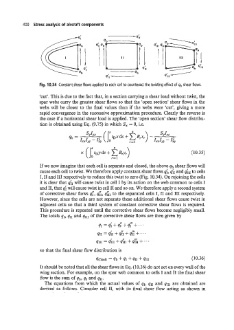
Fig. 10.34 Constant shear flows applied to each cell to counteract the twisting effect of q, shear flows.

‘cut’. This is due to the fact that, in a section carrying a shear load without twist, the
spar webs carry the greater shear flows so that the ‘open section’ shear flows in the
webs will be closer to the ha1 values than if the webs were ‘cut’, giving a more
rapid convergence in the successive approximation procedure. Clearly the reverse is
the case if a horizontal shear load is applied. The ‘open section’ shear flow distribu-
tion is obtained using Eq. (9.75) in which S, = 0, i.e.

(10.35)

If we now imagine that each cell is separate and closed, the above qb shear flows will
cause each cell to twist. We therefore apply constant shear flows 4, qfI and dII to cells
I, I1 and I11 respectively to reduce this twist to zero (Fig. 10.34). On rejoining the cells
it is clear that dI will cause twist in cell I by its action on the web common to cells I
and 11, that qi will cause twist in cell I1 and so on. We therefore apply a second system
of corrective shear flows 4, d1, dI1 to the separated cells I, I1 and I11 respectively.
However, since the cells are not separate these additional shear flows cause twist in
adjacent cells so that a third system of constant corrective shear flows is required.
This procedure is repeated until the corrective shear flows become negligibly small.
The totals qI, qII and qIII of the corrective shear flows are then given by
qI =d+d+qr(l+--
411 = 41 + a: + 4 + . . .

qIII = 411 + 411 + qYi1 + . . *
so that the final shear flow distribution is

q(fina1) = qb -k 41 + 411 + qIII (10.36)
It should be noted that all the shear flows in Eq. (10.36) do not act on every wall of the
wing section. For example, on the spar web common to cells I and I1 the final shear
flow is the sum of qb, qI and qII.
The equations from which the actual values of qI, qII and qIII are obtained are
derived as follows. Consider cell 11, with its final shear flow acting as shown in