Page 567 -

DECISION MAKING WITH PROBABILITIES 547

The expected value (EV) of decision alternative d i is defined as follows:

X
N
EVðd i Þ¼ Pðs j ÞV ij (13:4)
j¼1

In words, the expected value of a decision alternative is the sum of weighted payoffs
for the decision alternative. The weight for a payoff is the probability of the
associated state of nature and therefore the probability that the payoff will occur.
Let us return to the PDC problem to see how the expected value approach can be
applied.
PDC is optimistic about the potential for the complex. Suppose that this optimism
leads to an initial subjective probability assessment of 0.8 that demand will be strong
(s 1 ) and a corresponding probability of 0.2 that demand will be weak (s 2 ). Thus,
P(s 1 ) ¼ 0.8 and P(s 2 ) ¼ 0.2. Using the payoff values in Table 13.1 and equation
(13.4), we calculate the expected value for each of the three decision alternatives as
follows:
EVðd 1 Þ¼ 0:8ð8Þþ 0:2ð7Þ ¼ 7:8
EVðd 2 Þ¼ 0:8ð14Þþ 0:2ð5Þ ¼ 12:2
EVðd 3 Þ¼ 0:8ð20Þþ 0:2ð 9Þ¼ 14:2
Thus, using the expected value approach, we find that the large complex, with an
expected value of R14.2 million, is the recommended decision.
The calculations required to identify the decision alternative with the best
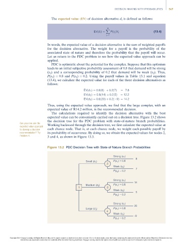
expected value can be conveniently carried out on a decision tree. Figure 13.2 shows
the decision tree for the PDC problem with state-of-nature branch probabilities.
Can you now use the
expected value approach Working backward through the decision tree, we first calculate the expected value at
to develop a decision each chance node. That is, at each chance node, we weight each possible payoff by
recommendation? Try its probability of occurrence. By doing so, we obtain the expected values for nodes 2,
Problem 4. 3 and 4, as shown in Figure 13.3.

Figure 13.2 PDC Decision Tree with State-of-Nature Branch Probabilities

Strong (s ) 8
1
1
Small (d 1 ) P(s ) = 0.8
2
Weak (s )
2
) = 0.2 7
P(s 2
Strong (s 1 )
14
Medium (d ) P(s ) = 0.8
1
2
1 3
Weak (s 2 )
5
P(s 2 ) = 0.2
Strong (s 1 )
20
Large (d ) P(s ) = 0.8
1
3
4
Weak (s ) –9
2
P(s ) = 0.2
2

Copyright 2014 Cengage Learning. All Rights Reserved. May not be copied, scanned, or duplicated, in whole or in part. Due to electronic rights, some third party content may be suppressed from the eBook and/or eChapter(s). Editorial review has
deemed that any suppressed content does not materially affect the overall learning experience. Cengage Learning reserves the right to remove additional content at any time if subsequent rights restrictions require it.