Page 429 - Analog and Digital Filter Design

426 Analog and Digital Filter Design

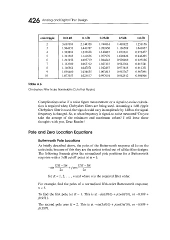
I orderkipple I O.OldB 0.ldB 0.25dB 0.5dB l.OdB

2 3.667181 2.144358 1.744861 1.488922 1.253156
3 1.964153 1.441787 1.282450 1.166589 1.041057
4 1.503881 1.232628 1.140487 1.065631 0.973477
5 1.311385 1.141656 1.077978 1.020826 0.943285
6 1.211956 1.093719 1.044843 0.996982 0.927166
7 1.153700 1.065312 1.025137 0.982764 0.917541
8 1.116561 1.047071 1.012457 0.973615 0.911331
9 1.091400 1.034655 1.003813 0.967367 0.907091
10 1.073553 1.025817 0.997654 0.962912 0.904066

Complications arise if a noise figure measurement or a signal-to-noise calcula-
tion is required when Chebyshev filters are being used. Assuming a 1 dB ripple
Chebyshev filter is used, the signal could vary in amplitude by 1 dB as the signal
frequency is changed. So, at what frequency is signal-to-noise measured? Do you
take the average of the minimum and maximum values? I will leave those
thoughts with you, Dear Reader!

Pole and Zero location Equations

Butterworth Pole locations
As briefly described above, the poles of the Butterworth response all lie on the
unit circle; because of this they are the easiest to find out of all the filter designs.
The following formula gives the normalized pole positions for a Butterworth
response with a 3 dB cutoff point at o = 1:

(2K - 1)7r (2K -1)~
-sin + jcos
212 2n
for K = 1, 2, . . . , n and where n is the required filter order.

For example, find the poles of a normalized fifth-order Butterworth response;
n = 5.
To find the first pole, let K= 1. This is at -sin(dlO) +jcos(dlO), or -0.309 +
~0.9511.
The second pole uses K= 2. This is at -sin(3d10) +jcos(3dlO), or -0.809 +
j0.5878.