Page 57 - Analog and Digital Filter Design

54 Analog and Digital Filter Design

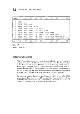
Order c1 L2 c3 L4 c5 L6 c7 L8 c9 L10
1 1.125
2 0.05889 I 1.768
3 1.5624 0.8608 0.2986
4 0.02705 5.0202 0.12546 12.929
5 1.6102 1.036 0.7598 0.4762 0.1634
6 0.01623 3.05343 0.07641 6.5521 0.1307 12.9068
7 1.6111 1.04312 0.84037 0.6797 0.5066 0.31384 0.10624
8 0.01 11 2.1008 0.05326 4.6079 0.08876 6.7381 0.12902 12.8264
9 1.6038 1.0251 0.8408 0.7241 0.6169 0.49904 0.36722 0.22512 0.07576
10 0.008 16 1.5566 0.03938 3.479 0.06766 5.08897 0.09093 6.6556 0.1267 12.774
Rs=% L1’ C2’ L3’ C4‘ L5’ C6‘ L7’ C8’ L9’ C10’

Butterworth Response

The Butterworth response has a smooth passband and a smooth increase in
stopband attenuation. It differs from the Bessel response in that the attenuation
in the stopband rises by n x 6dB/octave almost immediately outside the pass-
band. Figure 2.10 gives a graph showing how the attenuation rises with fre-
quency and filter order. A curve is given in the graph for each filter order up to
ten. Using the graph, it is possible to determine the filter order required to give
a certain level of attenuation at some multiple of the cutoff frequency.

For example, suppose the desired specification of a filter is that it has 60dB
attenuation at three times the cutoff frequency. Using Figure 2.10, the w= 3 axis
and 60dB attenuation axis cross at a point midway between the curves of n = 6
and n = 7. A seventh-order filter will meet the specification.