Page 117 - Applied Process Design For Chemical And Petrochemical Plants Volume III

66131_Ludwig_CH10C 5/30/2001 4:21 PM Page 84

84 Applied Process Design for Chemical and Petrochemical Plants

Many cooling waters have inverse solubility characteristics ©1978 by Gulf Publishing Company, all rights reserved. It is
due to dissolved salt compounds (organic and inorganic); based on: R t R* (1 e BT ). The asymptotic value, R*, is
others carry suspended solids that deposit on the tube at low- the expected fouling resistance after operating at time 2
flowing velocities ( 2 ft/sec). Biological fouling usually does and is the value proposed for the use in design.
not occur and is not a serious problem in most plant waters
that are treated with biocides. Inverse solubility of dissolved “In order to use these nomographs two sets of data have
salts in water occurs when the water contacts warm surfaces to be known: t 1 , R 1 , and t 2 , R 2 .
140
and the salts deposit on the tube surfaces . Do not design Prior to using these nomographs, the auxiliary values
an exchanger by selecting a fouling resistance that has not have to be computed:
fully developed, but rather select a value that has stabilized
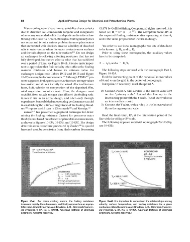
over a period of time, see Figure 10-41. It is also quite impor- t 1 >t 2 and R 1 >R 2
tant to appreciate that fluid velocity often affects the fouling
material thickness and hence its ultimate value for The following steps are used with the nomograph Part 1,
exchanger design; note Tables 10-12 and 10-13 and Figure Figure 10-43A.
10-42 as examples for some waters. 140 Although TEMA 107 pre- Find the intersecting point of the curves of known values
sents suggested fouling resistances, r, these are average values of and on the grid in the center of nomograph.
to consider and do not identify the actual effects of hot sur- Interpolate if necessary; mark this point A.
faces, fluid velocity, or composition of the deposited film,
solid suspension, or other scale. Thus, the designer must 2) Connect Point A, with a ruler, to the known value of
establish from usually meager data (if any) the fouling resis- on the “primary scale.” Extend this line up to the
tances to use in an actual design, and often only through intersecting point with the Y scale. (Read the Y value as
experience. Some field plant operating performance can aid an intermediate result).
in establishing the ultimate magnitude of the fouling. Knud- 3) Connect the Y value, with a ruler, to the known value of
sen 140 reports useful data in Chenoweth 142 and Koenigs. 141 R 1 on the appropriate scale.
Zanker 143 has presented a graphical technique for deter-
mining the fouling resistance (factor) for process or water Read the final result, R*, at the intersection point of the
fluid systems based on selected or plant data measurements, line with the oblique R* scale.
as shown in Figures 10-43A, 10-43B, and 10-43C. The design The following steps are used with nomograph Part 2 (Fig-
determination procedure presented by Zanker 143 is quoted ure 10-43B).
here and used by permission from Hydrocarbon Processing

Figure 10-41. For many cooling waters, the fouling resistance Figure 10-42. It is important to understand the relationships among
increases rapidly, then decreases, and finally approaches an asymp- velocity, surface temperature, and fouling resistance for a given
totic value. (Used by permission: Knudsen, J. G., Chemical Engineer- exchanger. (Used by permission: Knudsen, J. G., Chemical Engineer-
ing Progress. V. 87, No. 4, ©1991. American Institute of Chemical ing Progress. V. 87, No. 4, ©1991. American Institute of Chemical
Engineers. All rights reserved.) Engineers. All rights reserved.)