Page 133 - Cam Design Handbook

THB5 8/15/03 1:52 PM Page 121

CAM MOTION SYNTHESIS USING SPLINE FUNCTIONS 121

8

Acceleration (cm/rad/rad) 0

Splines
Polynomials
Constraint
–8
0 90 180 270
Cam rotation angle (deg.)
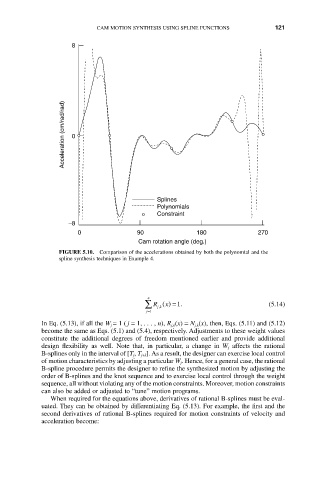
FIGURE 5.10. Comparison of the accelerations obtained by both the polynomial and the
spline synthesis techniques in Example 4.

n
 R () =1 . (5.14)
x
jk ,
j=1
In Eq. (5.13), if all the W j = 1 ( j = 1,... , n), R j,k (x) = N j,k (x), then, Eqs. (5.11) and (5.12)
become the same as Eqs. (5.1) and (5.4), respectively. Adjustments to these weight values
constitute the additional degrees of freedom mentioned earlier and provide additional
design flexibility as well. Note that, in particular, a change in W j affects the rational
B-splines only in the interval of [T j , T j+k ]. As a result, the designer can exercise local control
of motion characteristics by adjusting a particular W j . Hence, for a general case, the rational
B-spline procedure permits the designer to refine the synthesized motion by adjusting the
order of B-splines and the knot sequence and to exercise local control through the weight
sequence, all without violating any of the motion constraints. Moreover, motion constraints
can also be added or adjusted to “tune” motion programs.
When required for the equations above, derivatives of rational B-splines must be eval-
uated. They can be obtained by differentiating Eq. (5.13). For example, the first and the
second derivatives of rational B-splines required for motion constraints of velocity and
acceleration become: