Page 135 - Cam Design Handbook

THB5 8/15/03 1:52 PM Page 123

CAM MOTION SYNTHESIS USING SPLINE FUNCTIONS 123

placement. This expedient has no effect on the computations or conceptual basis. In prac-
(m)
th
tical applications, the actual displacement, Y, and its m derivative, Y , of the follower
can found from the normalized values as follows:
()
m
()
t
Y = S () ◊ h, Y () x () = S () ◊◊(w b ) .
t
m
h
m
c c c c
If time, t, starts at the beginning of the rise, then normalized time is t = t/T h , where T h is
the total time for the rise of h.
EXAMPLE 5: A Simple Case Illustrating the Effect of Varying the Weight Sequence
In this example, six boundary motion constraints for a follower system, listed in Table 5.5,
are used to define a DRD motion program for a cam. With these six motion constraints,
the velocities and accelerations of the cam will be continuous and will vanish at both ends
of the normalized time domain. The cam profile can be determined by geometric methods
(Hanson and Churchill, 1962) from the cam displacement curve and its derivatives. As
described earlier, to ensure continuous cam acceleration curve, at least, cubic rational B-
splines must be applied. In this example, the order k = 5 is chosen so the cam has a quad-
ratic acceleration curve. Hence, there is only one interior knot and it is placed at the
midpoint of the time domain for this example. (The effect of varying knots on the B-spline
method was illustrated in the earlier examples and so will not be repeated here.) To satisfy
these six constraints, six rational B-splines are constructed. This is done with the three
different weight sequences below to show the influence of this parameter.
Figures 5.11 to 5.13 show the series of rational spline functions that result from these
weight sequences. Since the first sequence consists only of values of unity, the rational B-
splines shown in Fig. 5.11 are identical to those that would be obtained by the B-spline
method. In Fig. 5.12, the rational B-splines located in the range of [0.5, 1.0] are per-
turbed by the variation of W 6 , which influences the basis functions constructed in the inter-
val of [T 6 , T 11 ]. This occurs, as can be seen from the equations, because the reduced value
of W 6 increases values for the fifth rational B-spline and decreases them for the sixth. As
a result, the cam displacement and its derivatives in Figs. 5.14 to 5.16 are affected only
in the range of [0.5, 1.0]. The change is small, illustrating the potential for exercising del-
icate local control over motion characteristics. The perturbed rational B-splines resulting
from the third series of weights is shown in Fig. 5.13. Also, Figs. 5.14 to 5.16 show that
the cam displacement and its derivatives are affected over the entire range [0.0, 1.0] and
that these effects are much more pronounced than those of the second series of weights.
The effect occurs over the entire range of motion because the affected spline functions
(splines 2, 3, 4, and 5) span the entire range.

EXAMPLE 6: Reduction of Peak Velocity and Acceleration by Adjusting the Weight
Sequence Example 5 demonstrated that varying the weight sequence affects the peak
values of the velocities and acceleration. The potential value of this characteristic will be
shown by considering a spring-return cam-follower system in which it is desired to reduce

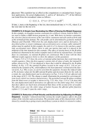
TABLE 5.5 Weight Sequences Used in
Example 5

[W] 1 = [1.0, 1.0, 1.0, 1.0, 1.0, 1.0]
[W] 2 = [1.0, 1.0, 1.0, 1.0, 1.0, 0.4]
[W] 3 = [1.0, 1.0, 1.0, 1.5, 1.0, 1.0]