Page 104 - Corrosion Engineering Principles and Practice

78 C h a p t e r 4 C o r r o s i o n T h e r m o d y n a m i c s 79

2

1.5
b
1
Potential (V vs. SHE) –0.5 0 a Al 3+ Al O ·H O AlO 2 –
0.5

2
3
2

–1

–1.5
Al
–2
–2 0 2 4 6 8 10 12 14 16
pH

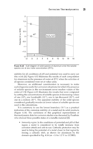
FIGURE 4.12 E-pH diagram of solid species of aluminum when the soluble
species are at one molar concentration (25°C).

stability for all conditions of pH and potential was used to carry out
this work [4]. Figure 4.12 illustrates the results of such computation
for aluminum in the presence of water at 25°C when the activities of
all species considered were set at value unity.
However, an additional consideration is necessary to make
such diagrams useful for corrosion situations for which the presence
of soluble species in the environment never reaches values of the
order of 1 M. Figure 4.13 illustrates the results that were computed
by setting the concentrations of soluble species at decreasing values
of one (10 ), one hundredth (10 ), one in ten thousand (10 ), and
−2
−4
0
one in a million (10 ). The apparent stability of the solid species
−6
considered gradually recedes as lower values of soluble species are
used in the calculations.
It is customary to use the lowest boundary (10 ) as a practical
−6
indication of the corrosion stability of a metal and its solid products
(Figure 4.14). The usefulness of this graphical representation of
thermodynamic data for corrosion studies was discussed by Pourbaix
who showed three possible states of a metallic material [3]:
• Immunity region: In the conditions of potential and pH of that
region a metal is considered to be totally immune from
corrosion attack and safe to use. Cathodic protection may be
used to bring the potential of a metal closer to that region by
forcing a cathodic shift, as shown for aluminum by the
domain specified in Fig. 4.14 (or −1.0 to 1.2 V vs. CCSRE).