Page 723 - Engineering Digital Design

14.5 STATE DIAGRAMS, K-MAPS, AND STATE TABLES FOR ASYNCHRONOUS FSMs 689

PS State
variable NS
change variable

Y,
y t
0^ 0 Stable 0 -» 0 0 -» 0 0
1 -» 0 Unstable 0 -> 1 Set 0 -» 1 1
0 -» 1 Unstable 1 -» 0 1 -> 0 0
1 -» 1 Stable 1 -> 1 Set Hold 1 -> 1 1

(a) (b) (c)
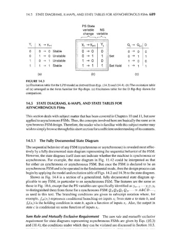
FIGURE 14.3
(a) Excitation table for the LPD model as derived from Eqs. (14.3) and (14.4). (b) The excitation table
of (a) arranged in the form familiar for flip-flops, (c) Excitation table for the D flip-flop shown for
comparison.

14.5 STATE DIAGRAMS, K-MAPS, AND STATE TABLES FOR
ASYNCHRONOUS FSMs

This section deals with subject matter that has been covered in Chapters 10 and 11, but now
applied to asynchronous FSMs. Thus, the concepts involved here are basically the same as in
synchronous FSM design. Therefore, the reader who is familiar with this subject matter may
wish to simply browse through this short section for a sufficient understanding of its contents.

14.5.1 The Fully Documented State Diagram
The sequential behavior of any FSM (synchronous or asynchronous) is revealed most effec-
tively by a fully documented state diagram representing the sequential behavior of the FSM.
However, the state diagram itself does not indicate whether the machine is synchronous or
asynchronous. For example, the state diagram in Fig. 11.42 could be interpreted as that
for either an synchronous or asynchronous FSM. But once the FSM is declared to be an
asynchronous FSM and to be operated in the fundamental mode, then the design process can
begin by applying the model and excitation table of Figs. 14.2 and 14.3b to the state diagram.
Shown in Fig. 14.4 is a section of a generalized, fully documented state diagram ap-
plicable to any FSM, in particular to an asynchronous FSM. The features are the same as
those in Fig. 10.6, except that the PS variables are specifically identified as y m-\ • • • j2j\ Jo
to distinguished them from those for a synchronous FSM QAQsQcQo • • • = ABCD • • •,
as used in this text. The branching conditions are given in subscript notation where, for
example, f ab(.Xi) represents conditional branching on inputs */ from state a to state b, and
fb(X{) is the holding condition in state b, again a function of inputs *,. Also, the output in
state c is conditional on some function of inputs x f .

Sum Rule and Mutually Exclusive Requirement The sum rule and mutually exclusive
requirement for state diagrams representing asynchronous FSMs are given by Eqs. (10.3)
and (10.4); the conditions under which they can be violated are discussed in Section 10.3.