Page 725 - Engineering Digital Design

14.5 STATE DIAGRAMS, K-MAPS, AND STATE TABLES FOR ASYNCHRONOUS FSMs 691

\Vi -Wo \Vp-i -Wo
y m-i ••• y p+iv\o-oo 0-01 0-11 - y m-i ••• y^vX Q-QQ.0-01
w
0---00 0-00
0
0---01 etc. 0-01 etc.

0-11 0-11

/Y k
(a) (b)
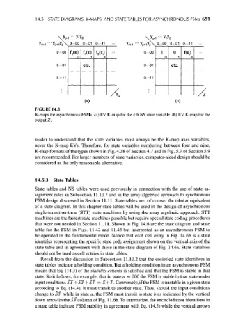
FIGURE 14.5
K-maps for asynchronous FSMs. (a) EV K-map for the /cth NS state variable, (b) EV K-map for the
output Z.

reader to understand that the state variables must always be the K-map axes variables,
never the K-map EVs. Therefore, for state variables numbering between four and nine,
K-map formats of the types shown in Fig. 4.38 of Section 4.7 and in Fig. 5.7 of Section 5.9
are recommended. For larger numbers of state variables, computer-aided design should be
considered as the only reasonable alternative.

14.5.3 State Tables
State tables and NS tables were used previously in connection with the use of state as-
signment rules in Subsection 11.10.2 and in the array algebraic approach to synchronous
FSM design discussed in Section 11.11. State tables are, of course, the tabular equivalent
of a state diagram. In this chapter state tables will be used in the design of asynchronous
single-transition-time (STT) state machines by using the array algebraic approach. STT
machines are the fastest state machines possible but require special state coding procedures
that were not needed in Section 11.11. Shown in Fig. 14.6 are the state diagram and state
table for the FSM in Figs. 11.42 and 11.43 but interpreted as an asynchronous FSM to
be operated in the fundamental mode. Notice that each cell entry in Fig. 14.6b is a state
identifier representing the specific state code assignment shown on the vertical axis of the
state table and in agreement with those in the state diagram of Fig. 14.6a. State variables
should not be used as cell entries in state tables.
Recall from the discussion in Subsection 11.10.2 that the encircled state identifiers in
state tables indicate a holding condition. But a holding condition in an asynchronous FSM
means that Eq. (14.3) of the stability criteria is satisfied and that the FSM is stable in that
state. So it follows, for example, that in state a = 000 the FSM is stable in that state under
input conditions ST + ST + ST = S + T. Conversely, if the FSM is unstable in a given state
according to Eq. (14.4), it must transit to another state. Thus, should the input conditions
change to ST while in state a, the FSM must transit to state b as indicated by the vertical
down arrow in the S f column of Fig. 11.6b. To summarize, the encircled state identifiers in
a state table indicate FSM stability in agreement with Eq. (14.3) while the vertical arrows