Page 432 - Excel 2007 Bible

26_044039 ch20.qxp 11/21/06 11:11 AM Page 389
Learning Advanced Charting
Working with the Legend
A chart’s legend consists of text and keys that make it easier to identify the data series. A key is a small
graphic that corresponds to the chart’s series (one key for each series).
To add a legend to your chart, choose Chart Tools ➪ Layout ➪ Labels ➪ Legend. This drop-down control
contains several options for the legend placement. After you’ve added a legend, you can drag it to move it
anywhere you like.
If you move a legend from its default position, you may want to change the size of the Plot
TIP
TIP
Area to fill in the gap left by the legend. Just select the Plot Area and drag a border to make it
the desired size.
The quickest way to remove a legend is to select the legend and then press Delete.
You can select individual items within a legend and format them separately. For example, you may want to
make the text bold to draw attention to a particular data series. To select an element in the legend, first
select the legend and then click the desired element.
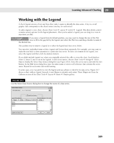
If you didn’t include legend text when you originally selected the cells to create the chart, Excel displays
Series 1, Series 2, and so on in the legend. To add series names, choose Chart Tools ➪ Design ➪ Select
Data to display the Select Data Source dialog box (see Figure 20.6). Select the series name and click the Edit 20
button. In the Edit Series dialog box, type the series name or enter a cell reference that contains the series
name. Repeat for each series that needs naming.
In some cases, you may prefer to omit the legend and use callouts to identify the data series. Figure 20.7
shows a chart with no legend. Instead, it uses Shapes to identify each series. These Shapes are from the
Callouts section of the Chart Tools ➪ Layout ➪ Insert ➪ Shapes gallery.
FIGURE 20.6
Use the Select Data Source dialog box to change the name of a data series.

389