Page 297 - Fair, Geyer, and Okun's Water and wastewater engineering : water supply and wastewater removal

JWCL344_ch07_230-264.qxd 8/2/10 8:44 PM Page 257

Problems/Questions 257

results for pipe P-1 show that the roughness value is much lower. This could indicate that a valve
is partially closed, the pipe is blocked, or that the pipe diameter may be smaller than expected. In
this case, pipe P-1 should be investigated to determine the cause of this low roughness value. If
there is a problem and that problem was fixed, new field measurements should be taken.
These roughness values can be entered into the model and further simulations can be con-
ducted. With enough field data, a model that closely simulates the actual system can be created.
Keep in mind that many times the person doing the modeling must decide what values to put into the
model. The software can only calculate values based on what is entered. The person doing the mod-
eling must judge how accurate the model is and whether the model can be used to make decisions.

PROBLEMS/QUESTIONS
Solve the following problems using the WaterGEMS computer Table 7.12 Junction Information for Problem 7.1
program.
Junction Demand (L/min)
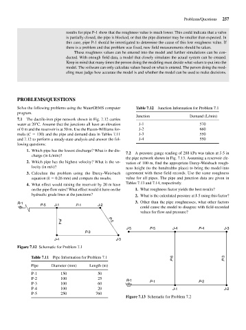
7.1 The ductile-iron pipe network shown in Fig. 7.12 carries
water at 20 C. Assume that the junctions all have an elevation J-1 570
of 0 m and the reservoir is at 30 m. Use the Hazen-Williams for- J-2 660
mula (C 130) and the pipe and demand data in Tables 7.11 J-3 550
and 7.12 to perform a steady-state analysis and answer the fol- J-4 550
lowing questions:
1. Which pipe has the lowest discharge? What is the dis-
7.2 A pressure gauge reading of 288 kPa was taken at J-5 in
charge (in L/min)?
the pipe network shown in Fig. 7.13. Assuming a reservoir ele-
2. Which pipe has the highest velocity? What is the ve- vation of 100 m, find the appropriate Darcy-Weisbach rough-
locity (in m/s)? ness height (to the hundredths place) to bring the model into
3. Calculate the problem using the Darcy-Weisbach agreement with these field records. Use the same roughness
equation (k 0.26 mm) and compare the results. value for all pipes. The pipe and junction data are given in
Tables 7.13 and 7.14, respectively.
4. What effect would raising the reservoir by 20 m have
on the pipe flow rates? What effect would it have on the 1. What roughness factor yields the best results?
hydraulic grade lines at the junctions? 2. What is the calculated pressure at J-5 using this factor?
R-1 3. Other than the pipe roughnesses, what other factors
P-5 J-1 P-1 J-2
could cause the model to disagree with field-recorded
values for flow and pressure?

P-2
P-4
J-5 P-5 J-4 P-4 J-3
P-3
J-4 J-3
Figure 7.12 Schematic for Problem 7.1

Table 7.11 Pipe Information for Problem 7.1 P-6 P-3

Pipe Diameter (mm) Length (m)
P-1 150 50
P-2 100 25
R-1 P-1 P-2
P-3 100 60
P-4 100 20 J-1 J-2
P-5 250 760
Figure 7.13 Schematic for Problem 7.2